In Part 3, we briefly discussed how Bayesian networks lead to compact representation of probabilistic models.
- Consider a model with N=4 variables, each of which has k possible values (0,1,...,k–1). How many different elementary events are there in the domain? One less is the number of probabilities that we'd have to determine in order to fully specify the model. (For example, in the Car model of Part 3, with N=6 and k=2, this number was 63.)
- How many parameters would we have to define to specify the model using an "empty" Bayesian network, i.e, a network with no edges at all?
- What is the maximum number of parameters we'd have to define in a Bayesian network in this domain (N variables with k values each)? Remember that the graph has to be a DAG, i.e., no directed cycles are allowed.
- Optional: Generalize to arbitrary values of N. It may be helpful to recall the sum of a geometric series 1+k+k2+...+kN–1 = (kN–1)/(k–1), where k≠1.
Implement an algorithm for generating data from the Car network
discussed in Part 3. You should generate n tuples, each of which is
a six element list of bits (or Boolean values). You should start by
choosing the value of B so that it takes value 1
(or True) with probability 0.9. After choosing the
value of B, choose the value of R. If B=0, then R=0 with probability
1. If B=1, then R=0 with probability 0.1. Continue this way,
choosing the probabilities from the CPTs, until you have generated a
complete tuple.
Generate a sample of n=100 000 tuples. Use it to approximate the following conditional probabilities:
- P(B | R,G,¬S)
- P(S | R,I,G)
- P(S | ¬R,I,G)
- Give an interpretation to the above probabilities. Are they in line with your intuition? In other words, do they make sense?
Consider the following scenario. You live in an area where earthquakes happen on the average every 111th day. Another annoying thing is that a burglar breaks into your home on the average once a year. Both events occur independently of each other and uniformly throughout the year (so any day is like another).
In case of an earthquake, your home alarm goes off with probability 0.81. If your home is broken into, the alarm goes off with probability 0.92. If these both should occur at the same time, the alarm goes off with probability 0.97. If nothing special is going on, there's a false alarm with probability 0.0095.
Now modify the algorithm from the previous exercise so that you can generate data from variables [E]arthquake, [B]urglar, [A]larm. Generate a sample of n=100 000 tuples.
- Among the tuples with A=1, what is the fraction where B=1?
- Among the tuples with A=1 and E=1, what is the fraction where B=1?
- Give an interpretation to your answers for items 1 & 2. What probabilities do they approximate?
- Are they in line with your intuition? In other words, do they make sense? In particular: which of the fractions is bigger and why?
- Repeat the experiment a couple of times to get a feeling of how much the results change just by chance. (This is the nature of the Monte Carlo approximation.) Experiment with different values of n. How does it affect the variability?
Machine Learning
| Theme | Objectives (after the course, you ...) | Machine learning |
|
Kinds of Machine Learning
It has been long understood that learning is a key element of intelligence. This holds both for natural intelligence -- we all get smarter by learning -- and artificial intelligence. In the latter case, learning is called machine learning.
The roots of machine learning are in statistics, which can also be thought of as the art of extracting knowledge from data. Especially methods such as linear regression and Bayesian statistics, which are both already more than two centuries old (!), are even today at the heart of machine learning. For a brief history, see the timeline of machine learning (Wikipedia).
The area of machine learning is often divided in subareas according to the kinds of problems being attacked. A rough categorisation is as follows:
- Supervised learning
- Unsupervised learning
- Reinforcement learning
- ...
We will focus primarily on supervised learning, and in particular, classification tasks. In classification, we observe in input, x, and try to infer its "class" y. There can be two or more possible class values. In the standard case, it is assumed that in each case, exactly one class value is "correct". In other words, it is not possible that an instance belongs to multiple classes (or none at all) at the same time. The training data is in the form of a set of (x,y) pairs.
Classification error means the fraction of incorrect classifications, i.e., cases where our classifier outputs the wrong class. It is important to keep in mind that the classification error can be quite different in the training data and a separate test set. This is related to the so called overfitting phenomenon. More about this very important topic on other courses such as Introduction to Machine Learning.
Good examples of classification tasks include: spam filtering (input is set of words in the message, class is spam/ham) and handwritten digit recognition (input is a bitmap image, class is 0,...,9).

Figure: Samples of handwritten images from the very commonly used MNIST dataset. The correct label (decided by a human) is shown above each image. Note that some of the "correct" class labels are questionable: see for example the second image from left: is that really a '7', or actually a '4'?
In this part, we'll study three classic and commonly used classifiers: first, the nearest neighbor classifier, second, the naive Bayes classifier (which is already familiar to you from the spam filter in Part 3), and third, the perceptron neural network classifier.
k-Nearest Neighbor (k-NN) Classifier
The nearest neighbor (NN) classifier is among the simplest possible classifiers. In the training stage, if you can call it that, all the training data is simply stored. When given a new instance, x(test), we find the training data point x(NN) which is closest to x(test) and output its class label y(NN) as the predicted class label. An example is given in the following diagram (panels a and b).
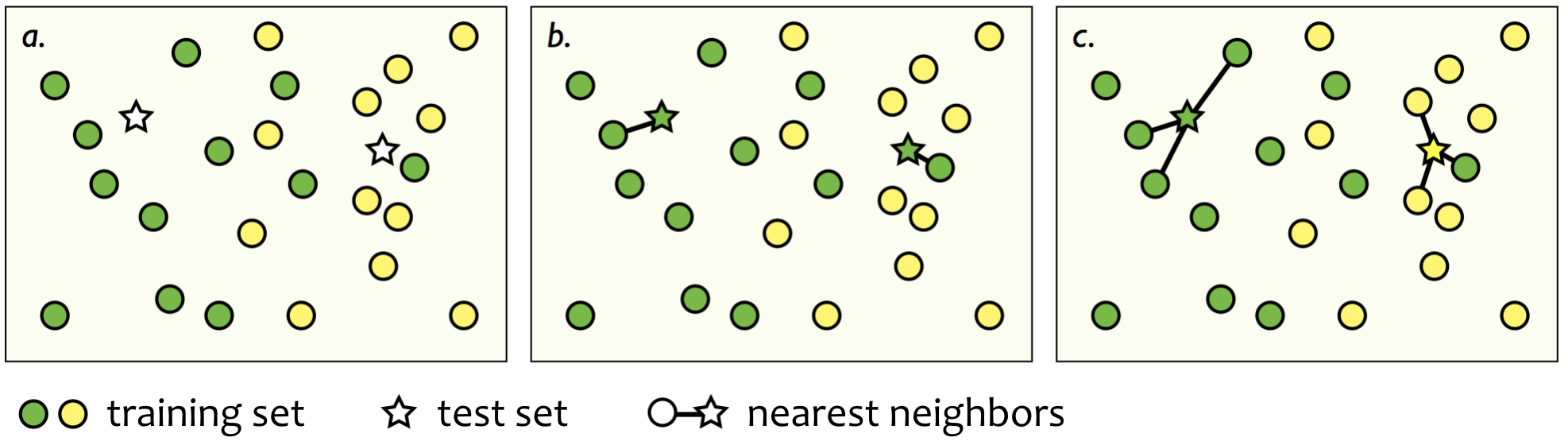
In the k-nearest neighbor (k-NN) classifier, the idea is very similar but here it is not only the single nearest point that is used. Instead, we find the k nearest training data points, and choose the majority class among them as the predicted label. This is illustrated in panel c of the above diagram.
An interesting question related to (among other things) the NN classifier is the definition of distance or similarity between instances. In the illustration above, we implicitly assumed that the Euclidean distance is used. However, this may not always be reasonable or even possible: the type of the input x may be, e.g., a string of characters (of possibly different lengths).
You should therefore choose the distance metric on a case-by-case basis. In the MNIST digit recognition case, we discussed the potential problems due to defining image similarity by counting pixel-by-pixel matches -- this was concluded to be sensitive to shifting or scaling the images. Fortunately, the MNIST data has been preprocessed by centering and scaling the images to alleviate some of these issues.
Naive Bayes Classifier
The naive Bayes classifier is actually already familiar to you from the spam filter problem in Part 3. Here we will see how the same idea can be applied to handwritten digit recognition. In the spam filter application, the class variable was binary (spam/ham) and the feature variables were the words in the message. In the digit recognition application, the class variable has ten different values (0,...,9), and the feature variables are the 28 × 28 = 784 pixel values (binary black/white) in the bitmap images. We store the pixel values in a single vector and use the value Xj=1 to indicate that the j'th pixel is white. The value Xj=–1 is used for the black color for convenience.
Here too, the feature variables are assumed to be independent of
each other given the class value, i = 0,...,9. In the training
stage, the algorithm estimates the conditional probabilities of each
pixel being white in an image of class i for each class and each
pixel. In the same manner as in the spam filter case, these
probabilities can be estimated as empirical frequencies:
P(Xj = 1 | Class = i) = #{Xj=1, Class=i} /
#{Class=i},
where #{Xj = 1, Class=i} is the number of training instances
of class i where the j'th pixel is white, and #{Class=i} is the
overall number of class i instances.
This estimator is implemented by the following pseudocode:
train_NB(data):
1:  for each class i in 0,...,9:
2:     model.prior[i] = #{class=i} / n
3:     for each pixel j in 0,...,783:

4:        model.cpt[i,j] = #{Xj=1, class=i} / #{class=i}
5:  return model
The estimated values are stored as the array cpt in
a model object. The array prior stores
the estimates of the probabilities P(Class=i) for all i=0,...,9.
Given a new image with pixel values
x0,...,x783 (so, for example, –1,–1,–1,1,... if the first
three pixels are black and the fourth is white, etc) the classifier computes
the joint probability
P(Class=i, X0=x0,...,X783=x783)
= P(Class=i) P(X0=x0 | Class=i) × ...
× P(X783=x783 | Class=i)
for all i=0,...,9.
The sum of these probabilities over the ten class values,
Z, is the annoying denominator in the Bayes rule, so we can obtain
the posterior probabilities by dividing the above joint
probabilities by Z:
P(Class=i | X0=x0,...,X783=x783)
= P(Class=i) P(X0=x0 | Class=i) × ...
× P(X783=x783 | Class=i) / Z
Pseudocode for doing computing the posterior probabilities is below.
posterior_NB(model, image):
1:  Z = 0; posterior = empty array

2:  for each class i in 0,...,9:
3:     posterior[i] = model.p[i]
4:     for each feature j in 0,...,783:

5:        if image[j] = 1:
6:           posterior[i] = posterior[i] * model.cpt[i,j]
7:        else:
8:           posterior[i] = posterior[i] * (1-model.cpt[i,j])
9:     Z = Z + posterior[i]
10: for each class i in 0,...,9:
11:    posterior[i] = posterior[i] / Z
12: return posterior
Note that since the pixels can only take one of two possible values (white or black), the probability of a pixel being black is obtained as one minus the probability of a white pixel (line 8 in the pseudocode).
To obtain a classifier that outputs a single class value, instead of the full posterior probability, we can pick the maximum a posteriori class value, i.e., the most probable class.
Neural Networks
Our next topic tends to attract more interest than many of the other topics on this course. Perhaps it is the hope to understand out own mind, which emerges from neural processing in our brain, that makes neural networks so interesting.
What is so Special about Neural Networks?
The case for neural networks as an approach to AI is based on a similar argument as that for logic-based approaches. In the latter case, it was (or is) thought that in order to achieve human-level intelligence, we need to simulate higher-level thought processes, and in particular, manipulation of symbols representing certain concrete or abstract concepts using logical rules. The argument for neural computation is that by simulating the lower-level, subsymblic data processing on the level of neurons and neural networks, intelligence will emerge.
Neural computation can even be thought to be an alternative to the conventional model of computation based on Turing machines. The main distinguishing features of neural computation compared to conventional computing are:
- parallelism: many neurons act simultaneously
- stochasticity: the behavior of neurons cannot be predicted in a deterministic fashion -- the same input can lead to different outputs
- massive scale: neural networks can involve hundreds of billions (1011) connections -- which is still 10000 times less than the estimated number of connections in the brain, 1015
- adaptivity: the connections have an inherent tendency to adapt over time
Artificial neural networks (ANNs) mimic natural neural networks by copying the basic idea of a connected system including a large number of simple processor units (neurons), where processing is carried out by transmitting signals between the neurons. However, the internal mechanism of the neurons is usually ignored and the artificial neurons are often much simpler than their natural counterparts. Likewise, the eletro-chemical signalling mechanisms between natural neurons are mostly ignored in the design of ANNs.
There are attempts to simulate natural neural networks. Perhaps most famously the Blue Brain Project for modelling the rat brain, and most infamously, the Human Brain Project, which promised about 10 years ago that "the mysteries of the mind can be solved -- soon". The Human Brain Project turned out to be based more on empty promises with the goal of raising a billion dollars rather than solid scientific evidence.
Most of the time, however, the goal is not to simulate a natural neural network but to implement AI and machine learning solutions. To build working solutions, it is not essential to replicate the details. In practice, we usually build ANNs that differ from natural neural networks in at least the following ways:
- computation in ANNs usually synchronous: all neurons complete their computation cycle before the proceeding to the next iteration, whereas natural systems tend to be asynchronous
- signaling in ANNs is usually continuous-valued as opposed to the binary (on/off or fire/don't fire) signals between natural neurons
- natural neural networks exhibit complex feedback loops -- only specialized ANNs known as recurrent networks have this feature (see below)
- ANNs are often much smaller in scale than natural nervous systems
Weights, Activation and Adaptation
The basic artificial neuron model involves a set of adaptive
parameters, called weights. These weights are used as
multipliers on the inputs of the neuron. We denote the
weighted sum of the inputs as:
z = Σj=1,...,n wj xj,
where n is the number of inputs. The weights are
real-valued, and the inputs can be either binary or real-values.
The output of the neuron is obtained by applying an activation function on the weighted sum z. Typical examples is the activation function include:
- step function: f(z) = –1, if z < 0, and 1 otherwise
- sigmoid function: f(z) = 1/(1+e–z)
The output of a neuron can then act as the input of other neurons, whose outputs can be the input to yet other neurons, etc. The output of the whole network is obtained as the output of a certain subset of the neurons, which are called the output layer, although not all neural architectures can be divided in such a way.
Learning or adaptation in the network occurs when the weights are adjusted so as to make the network produce the correct ouputs. Optimizing the weights manually is out of the question and learning ANNs is a machine learning problem. Even as a machine learning problem, the optimization problems in ANNs are among the hardest.
In the following, we will study three different kinds of neural networks:
- feedforward networks, where the information always flows in one diretion (from an input layer toward an output layer)
- recurrent networks, which include feedback loops
- the self-organizing map
Feedforward Networks
The simplest kind of ANNs from the point of view of their theoretical analysis are feedforward networks. Often the network architecture is composed of layers. The input layer consists of neurons that get their inputs directly from the data. So for example, in an image recognition task, the input layer would use the pixel values of the input image as the inputs of the input layer. The network typically also has hidden layers that use the other neurons' outputs as their input, and whose output is used as the input to other layers of neurons. Finally, the output layer produces the output of the whole network. All the neurons on a given layer get inputs from neurons on only a single (lower) layer.
We will return to multilayer networks in a little while, but first we'll study the simplest possible neural "network" which consists of a single neuron.
Perceptron: The Mother of all ANNs
A perceptron is a feedforward neural network that consists of a single basic neuron. It was among the very first formal models of neural computation and because of its fundamental role in the history of neural networks, it wouldn't be unfair to call it the "Mother of all Artificial Neural Networks". It can be used as a simple classifier in binary classification tasks. A classic neural network method is the Perceptron algorithm, introduced by Rosenblatt in 1957, which can be used to train a perceptron.
The perceptron neuron is simply the above basic neuron model with the step function as the activation function.
In the Perceptron algorithm, for which pseudocode is given below, each misclassification leads to an update in the parameter vector w. If the predicted output of the neuron is 1 when the correct class is y=–1, then the input vector x is subtracted from the weight vector. Similarly, if the predicted output is –1 when the correct class is y=1, then the input vector x is added to the weight vector. (Recall that vector subtraction and addition simply means the element-wise subtraction or addition of the two vectors.)
perceptron(data):

1:  w = [0, ...,0]               # array of size p
2:  while error(data, w) > 0:
3:     (x,y) = choose_random_item(data)
4:     z = w[0]x[0] + ... + w[p-1]x[p-1]
5:     if z ≥ 0 and y = -1:      # -1 classified as 1
6:        w = w − x              # subtract vector x
7:     if z < 0 and y = 1:       # 1 classified as -1
8:        w = w + x              # add vector x
9:  return(w)
In practice, it is impractical to choose random training data points on line 3 of the algorithm because this may lead to choosing correctly labeled examples most of the time, which is a waste of time since they lead to no updates in the weights. Instead, a better method is to iterate through the training data and as soon as a misclassified item is found, do the required update.
It can be theoretically proven that if the data is linearly separable, then the algorithm is guaranteed to stop after a finite number of steps and produce a weigth vector that correctly classifies all the training instances.
Use the Perceptron template on TMC. (You can also implement your solution in other languages than Java. You'll find the necessary data files in the TMC template.)
The file mnist-x.data contains 6000 images from the popular
MNIST dataset, each
of which is given on a single line in the file. Each image consists
of 28 × 28 pixels listed row-by-row, so each line in the file
contains 784 values. Each pixel is either black (–1) or white
(1). The file
mnist-y.data contains the correct class value (0-9) of each
of the 6000 images.
Use the first 5000 images as training data and the last 1000 as test data.
-
Run the Java template to make sure that the file
test100.bmpis created. It should include the first 100 images sorted according to the correct class label. This verifies that reading the file was successful. -
Modify the
train()method in classPerceptronso that it learns to distinguish number 3 from number 5. (Notice that the variabletargetCharcan be set to be one of these classes whileoppositeCharshould be the other. This will set the class label as 1 and –1 as is required in the Perceptron algorithm. Images representing other numbers are ignored.) Try to get a classification error around 5–15 %. - Try other pairs of number than 3 vs 5. Which numbers are easiest to classify and which are the hardest?
Now implement a nearest neighbor classifier for the MNIST data used in the Perceptron exercise.
Recall that unlike the Perceptron, or most other classifiers, the nearest neighbor classifier doesn't really involve a training stage. All the action happens in the classification (testing) stage. This style of methods are sometimes called "lazy learning": thou shalt not let it be your inspiration in real life!
Test your classifier using the same train/test split (5000/1000) as before. You can use the same pairs of numbers (3 vs 5), or even try classifying all the classes at the same time because the NN classifier is not restricted to binary classification. (Note that in multiclass classification, the expected accuracy tends to be lower than in binary classification simply because the problem is harder.)
Multilayer perceptrons
The main problem with the Perceptron algorithm is the assumption that the data are linearly separable. In practice, this tends not to be the case, and various variants of the algorithm have been proposed to deal with this issue. Two main directions are:
- Applying a non-linear transformation on the original input data may produce a representation where the data are linearly separable. The so called "kernel trick" leads to a class of methods known collectively as kernel methods, among which the support vector machine (SVM) is the best known.
- The model can be extended by coupling a number of basic neurons together to obtain neural networks that can represent complex, non-linear decision boundaries. A classical example of this is the multilayer perceptron (MLP).
An illustration showing that the second option leads to non-linear decision boundaries is given by the following video:
- Vimeo: Two Spirals Problem
Optimizing the weights of a multilayer perceptron is much harder than optimizing the weigths of a single perceptron neuron. The second coming of neural networks in the late 1980s was largely due to the difficulties faced by the then prevailing logic-based approach (so called expert systems) but also due to the invention of the backpropagation algorithm in the 1970s-1980s.
The path(s) leading to the backpropagation algorithm are rather long and winding. An interesting part of the history is related to the CS department of the University of Helsinki. About three years after the founding of the department in 1967, a Master's thesis was written by a student called Seppo Linnainmaa. The topic of the thesis was "Cumulative rounding error of algorithms as a Taylor approximation of individual rounding errors" (the thesis was written in Finnish, so this is a translation of the actual title "Algoritmin kumulatiivinen pyöristysvirhe yksittäisten pyöristysvirheiden Taylor-kehitelmänä").
The automatic differentiation method developed in the thesis was later applied by other researchers to quantify the sensitivity of the output of a multilayer neural network with respect to the individual weights, which is the key idea in backpropagation.
After its discovery, the Perceptron algorithm received a lot of attention, not least because of optimistic statements made by its inventor, Frank Rosenblatt. A classic example of AI hyperbole is a New York Times article published on July 8th, 1958:
The history of the debate that eventually lead to almost complete abandoning of the neural network approach in the 1960s for more than two decades is extremely fascinating. The article "A Sociological Study of the Official History of the Perceptrons Controversy" by Mikel Olazaran (Social Studies of Science, 1996) reviews the events from a sociology of science point of view. Reading it today is quite thought provoking -- and slightly chilling. Take for example a September 29th 2017 article in the MIT Technology Review, where Jordan Jacobs, co-founder of a multimillion dollar Vector institute for AI compares Geoffrey Hinton (a figure-head of the current deep learning boom) to Einstein because of his contributions to the discovery of the power of the backpropagation algorithm in the 1980s and later.The Navy revealed the embryo of an electronic computer today that it expects will be able to walk, talk, see, reproduce itself and be conscious of its existence. Later perceptrons will be able to recognize people and call out their names and instantly translate speech in one language to speech and writing in another language, it was predicted.
According to Hinton and Jacobs, we are on the brink of the final breakthrough. Sound familiar?
Please note that neural network enthusiasts are not at all the only ones inclined towards optimism. The rise and fall of the logic-based "expert systems" approach to AI had all the same hallmark features of an AI-hype, including promising results in restricted domains, gullible journalists, clueless investors in their cabinets, and too much speed to notice how "minor obstacles" were piling up and becoming big problems. The outcome both in the early 1960s and late 1980s was a collapse in the research funding, "AI Winter".
Recurrent Neural Networks
As stated above, recurrent neural networks involve feedback loops so they cannot be organized in an input layer, a number of hidden layers, and an output layer.
A classic example of this class of networks is the Hopfield network. In a Hopfield network, the neurons are binary (–1 or 1) and they are connected to each other by symmetric associative weights wi,j, which characterizes the strength of the association between neurons i and j. The association can be either positive or negative.
In the learning stage, a number of joint states of all the neurons
are used as training data, and the weights are fixed based on the
number of times a pair of neurons are in the same state in the
training data. The learning rule is given by
wi,j = Σk=1,...,n qik
qjk / n,
where qik=1 if neuron i is in state 1 in training example
k, and qik=–1 otherwise.
The neuron states can be given, for example, by pixels in a black-and-white image like in the MNIST task.
After the learning stage, the network can be initialized by setting the neuron states in specific states. However, the neurons are not fixed to these states, but they are allowed to choose new states according to the current states of the other neurons and the associative weights wi,j. The specific learning rule is in fact the very same as the one used in the perceptron neuron, i.e., a linear combination of the other neurons states weighted by the weights passed through a step function.
After all neurons have chosen their new state according to this rule, the same process is repeated so that the inputs of the neurons are given by the chosen new states. The process tends to converge rapidly to a fixed point which can be taken as the output of the network.
The Hopfield network can be used to implement an associative memory that retrieves typical patterns appearing in the training data given a partial match in the initial configuration. In practice, the Hopfield network is more significant as a conceptual model of how human or animal memory works than a technical tool for practical tasks.
A practically more relevant ANN model is the Boltzmann machine which is essentially a stochastic version of the Hopfield network. The main differences include the fact that the states of only a part of the neurons need to be given in the training data, and the learning and activation rules are different.
An nice illustration of using the Boltzmann machine to reconstruct incomplete images is given in the following video:
- Vimeo: The Shape Boltzmann Machine
The learning objectives related to neural networks are on a relatively high level: you should understand the basic idea (the learning method and the activation principles) in different kinds of ANNs. You should also learn what their main applications are. An exception is the perceptron classifier, which you should study in more detail -- that's why there is an exercise about it.
The Self-Organizing Map (SOM)
A third category or ANNs is the self-organizing map (SOM). In fact, this "category" is really made of a single method, developed by the Finnish neural network pioneer Teuvo Kohonen in the early 1980s.
The neurons in a SOM are organized in a regular two-dimensional grid. Each neuron has a weight or state vector. When an input, which is in the form of the same kind of vector as the state vectors, is presented, the neuron whose state vector is closest (in Euclidean distance) to the input vector is activated. This neuron is called the "winner". The learning rule modifies the state of the winner so that it becomes even more similar to the input vector. An important feature of the learning procedure is that also the neurons that are next to the winner in the grid, which we call the neighbors of the winner, are modified in a similar fashion.
A consequence of the learning procedure is that the state vectors of neurons that are located near each other in the grid tend to become more and more similar. Eventually, the result is a map where similar inputs activate nearby neurons. A typical application of the SOM is data visualization.