This week's first exercise is a continuation of the TravelPlanner from last week. The only difference is the change of algorithm: instead of breadth-first search, you should now implement A* search.
The cost associated with each transition from one stop to the next is the time required for the transition. This includes both the time spent waiting for the tram and the actual travel time. In our imaginary scenario, all trams leave at regular 10 minute intervals from their first stop (each line is given both ways, so another tram will leave at the same time from the other end).
Your route query will be given in the form:
TravelPlanner.search(departureStop, destinationStop, departureTime)
where the departure time can be given in minutes since the last full
10 minutes since the timetable of our tram network is so regular.
You'll need to complete the following steps (these instructions apply directly to Java but the general idea is the same in other languages):
- Implement a
StateComparatorclass (the Java package already has a template for this) with methodheuristic(Stop s), which calculates a lower bound on the time required to reach the destination from stops. A lower bound can be obtained by computing the distance between the two stops, and dividing it by the maximum speed of the tram which you can assume to be 260 coordinate points per minute. - Also implement method
compare(State s1, State s2)in classStateComparatorso that it can be used to order the nodes in the priotity queue based oncost + h(node)as described in Part 1. Here the nodes are states that are defined by the stop and the time since departure. - Implement the A* search in class
TravelPlanner. ThePriorityQueuedata structure comes in handy. An instance of theStateComparatorclass should be given as an argument to thePriorityQueueconstructor.
As before, you should return the obtained route as a backward-linked list of states.
The Stop class in the Java package provides
functionality for listing the neighboring stops and for getting the
minimum time required to get there (including the waiting time).
If you prefer to not use the Java package and TMC, that's totally
fine. You'll find the stop information in network.json
and the route descriptions in lines.json, both of which
are self-explanatory.
Games
This week, we will study a classic AI problem: games. The simplest scenario, which we will focus on for the sake of clarity, are two-player, perfect-information games such as tic-tac-toe and chess.
Another topic that we'll be able to get started with, and continue on next week, is reasoning under uncertainty using probability.
| Theme | Objectives (after the course, you ...) |
|---|---|
| Games and search (continued from last week) |
|
| Reasoning under uncertainty (to be continued next week) |
|
Games
Maxine and Minnie are true game enthusiasts. They just love games. Especially two-person, perfect information games such as tic-tac-toe or chess.
One day they were playing tic-tac-toe. Maxine, or Max as her friends call her, was playing with X. Minnie, or Min as her friends call her, had the Os. The situation was
       O| |O
       -+-+-
       X| |
       -+-+-
       X|O|
Max was looking at the board and contemplating her next move, as it
was her turn, when she suddenly buried her face in her hands in
despair, looking quite like Garry Kasparov playing Deep Blue in
1997.
Yes, Min was close to getting three Os on the top row, but Max could easily put a stop to that plan. So why was Max so pessimistic?
Game Trees
To analyse games and optimal strategies, we will introduce the concept of a game tree. The game tree is similar to a search tree, such as the one in the Sudoku example discussed at the lecture. (Remember that you should also study the lecture slides in addition to this material. Some material may be discussed in one but not the other.) The different states of the game are represented by nodes in the game tree. The "children" of each node N are the possible states that can be achieved from the state corresponding to N. In board games, the state of the game is defined by the board position and whose turn it is.
Consider, for example, the following game tree which begins
not at the root but in the middle of the game (because otherwise,
the tree would be way too big to display).
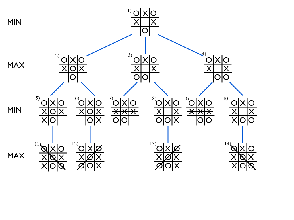
The game continues at the board position shown in the root node,
numbered as (1) at the top, with Min's turn to place O at any of the
three vacant cells. Nodes (2)--(4) show the board positions
resulting from each of the three choices respectively. In the next
step, each node has two possible choices for Max to play X each,
and so the tree branches again.
The game ends when either player gets a row of three, or when there are no more vacant cells. When starting from the above starting position, the game always ends in a row of three.
Now consider nodes (5)--(10) on the second layer from the bottom. In nodes (7) and (9), the game is over, and Max wins with three X's in a row. In the remaining nodes, (5), (6), (8), and (10), the game is also practically over, since Min only needs to place her O in the only remaining cell to win. We can thus decide that the end result, or the value of the game in each of the nodes on the second level from the bottom is determined. For the nodes that end in Max's victory, we'll say that the value equals +1, and for the nodes that end in Min's victory, we'll say that the value is -1.
More interestingly, let's now consider the next level of nodes towards the root, nodes (2)--(4). Since we decided that both of the children of (2), i.e., nodes (5) and (6), lead to Min's victory, we can without hesitation attach the value -1 to node (2) as well. For node (3), the left child (7) leads to Max's victory, +1, but the right child (8) leads to Min winning, -1. However, it is Max's turn to play, and she will of course choose the left child without hesitation. Thus, every time we reach the state in node (3), Max wins. Thus we can attach the value +1 to node (3).
The same holds for node (4): again, since Max can choose where to put her X, she can always ensure victory, and we attach the value +1 to node (4).
So far, we have decided that the value of node (2) is -1, which means that if we end up in such a board position, Min can ensure winning, and that the reverse holds for nodes (3) and (4): their value is +1, which means that Max can be sure to win if she only plays her own turn wisely.
Finally, we can deduce that since Min is an experienced player, she can reach the same conclusion, and thus she only has one real option: give Max an impish grin and play the O in the middle of the board.
In the diagram below, we have included the value of each node as
well as the optimal game play starting at Min's turn in the root
node.
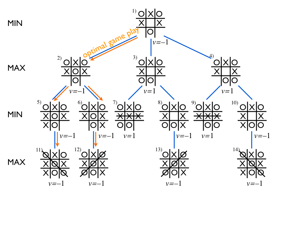
The value of the root node, which is said to be the value of the game, tells us who wins (and how much, if the outcome is not just plain win or lose): Max wins if the value of the game is +1, Min if the value is -1, and if the value is 0, then the game will end in a draw. This all is based on the assumption that both players choose what is best for them.
The optimal play can also be deduced from the values of the nodes: at any Min node, i.e., node where it is Min's turn, the optimal choices are given by those children whose value is minimal, and conversely, at any Max node, where it is Max's turn, the optimal choices are given the the children whose value is maximal.
Minimax Algorithm
We can exploit the above concept of the value of the game to obtain an algorithm with optimal game play in, theoretically speaking, any deterministic, two-person, perfect-information game. Given a state of the game, the algorithm simply computes the values of the children of the given state and chooses the one that has the maximum value if it is Max's turn, and the one that has the minimum value if it is Min's turn.
The algorithm can be implemented using the neat recursive functions below for Max and Min nodes respectively. This is known as the Minimax algorithm (see Wikipedia: Minimax).
1:  max_value(node):
2:     if end_state(node): return value(node)
3:     v = -Inf
4:     for each child in node.children():
5:        v = max(v, min_value(child))
6:     return v
1:  min_value(node):
2:     if end_state(node): return value(node)
3:     v = +Inf
4:     for each child in node.children():
5:        v = min(v, max_value(child))
6:     return v
Let's return to the tic-tac-toe game described in the beginning of this section. To narrow down the space of possible end-games to consider, we can observe that Max must clearly place an X on the top row to avoid imminent defeat:
       O|X|O
       -+-+-
       X| |
       -+-+-
       X|O|
Now it's Min's turn to play an O. Evaluate the value of this state
of the game as well as the other states in the game tree where the
above position is the root, using the Minimax algorithm.
As stated above, the Minimax algorithm can be used to implement optimal game play in any deterministic, two-player, perfect-information game. Such games include tic-tac-toe, connect four, chess, Go, etc. (Rock-paper-scissors is not in this class of games since it involves information hidden from the other player; nor are Monopoly or backgammon which are not deterministic.) So as far as this topic is concerned, is that all folks, can we go home now?
The answer is that in theory, yes, but in practice, no. In many games, the game tree is simply way too big to traverse in full. For example, in chess the average branching factor, i.e., the average number of children (available moves) per node is about 35. That means that to explore all the possible scenarios up to only two moves ahead, we need to visit approximately 35 x 35 = 1225 nodes -- probably not your favorite pencil-and-paper homework exercise... A look-ahead of three moves requires visiting 42875 nodes; four moves 1500625; and ten moves 2758547353515625 (that's about 2.7 quadrillion) nodes.
In Go, the average branching factor is estimated to be about 250. Go means no-go for Minimax.
Next, we will learn a few more tricks that help us manage massive game trees, and that were crucial elements in IBM's Deep Blue computer defeating the chess world champion, Garry Kasparov, in 1997.
Depth-limited minimax and heuristic evalution criteria
If we can afford to explore only a small part of the game tree, we need a way to stop the minimax recursion before reaching an end-node, i.e., a node where the game is over and the winner is known. This is achieved by using a heuristic evaluation function that takes as input a board position, including the information about which player's turn is next, and returns a score that should be an estimate of the likely outcome of the game continuing from the given board position.
Good heuristics for chess, for example, typically count the amount of material (pieces) weighted by their type: the queen is usually considered worth about two times as much as a rook, three times a knight or a bishop, and nine times as much as a pawn. The king is of course worth more than all other things combined since losing it amounts to losing the game. Further, occupying the strategically important positions, e.g., near the middle of the board, is considered an advantage.
The minimax algorithm presented above requires minimal changes to obtain a depth-limited version where the heuristic is returned at all nodes at a given depth limit.
Alpha-beta pruning
Another breakthrough in game AI, proposed independently by several researchers including John McCarthy in and around 1960, is alpha-beta pruning. For small game trees, it can be used independently of the heuristic evaluation method, and for large trees, the two can be combined into a powerful method that has dominated the area of game AI for decades.
A good example of the idea behind alpha-beta-pruning can be seen in the tic-tac-toe game tree that we discussed above -- scroll up and let the image of the root node burn into your retina.
Now simulate the Minimax algorithm at the stage where the value of
the left child node, -1, has been computed and returned to the
min_value function. The next step would be to
call max_value to compute the value of the middle
child. But hold on! If the left child guarantees victory for Minnie,
what does it matter how the game ends if she chooses to play any
other way? As soon as the algorithm finds a child node with the best
possible outcome for the player whose turn it is, it can make a
choice and avoid computing the values of all the other child nodes.
To implement this in a similar fashion as the Minimax algorithm
requires small changes in the min_value and
max_value functions. Understanding the connection
between these changes and the principle illustrated by the above
pruning example is not as easy as it may sound, so please pay
close attention to this topic and work out the examples and
exercises with care.
1:  max_value(node, alpha, beta):
2:     if end_state(node): return value(node)
3:     v = -Inf
4:     for each child in node.children():
5:        v = max(v, min_value(child, alpha, beta))
6:        alpha = max(alpha, v)
7:        if alpha >= beta: return v
8:     return v
1:  min_value(node, alpha, beta):
2:     if end_state(node): return value(node)
3:     v = +Inf
4:     for each child in node.children():
5:        v = min(v, max_value(child, alpha, beta))
6:        beta = min(beta, v)
7:        if alpha >= beta: return v
8:     return v
An important thing to remember is that the alpha value
is updated only at the Max nodes, and the beta value is
updated only at the Min nodes. The updated values are passed as
arguments down to the children, but not up to the calling parent
node. (That is, the arguments are passed as values, not as
references in programming lingo.)
The interpretation alpha and beta is that
they provide the interval of possible values of the game at the node
that is being processed:
alpha ≤ value ≤ beta. This interval
is updated during the algorithm, and if at some point, the interval
shrinks so that alpha = beta, we know the value and
can return it to the parent node without processing any more
child nodes. It can also happen that alpha > beta,
which implies that the current node will never be visited in
optimal game play, and its processing can likewise be aborted.
When starting the recursion at the root node, we use the minimum and
maximum value of the game as the alpha
and beta values respectively. For tic-tac-toe and
chess, for instance, where the outcome is plain win/loss, this
is alpha = -1 and beta = 1. If the range
of possible values is not specified in advance, we initialize
as alpha = -∞ and beta = ∞.
It is useful to work out a few examples to really understand the
beauty of alpha-beta pruning. Here's another tic-tac-toe
example.
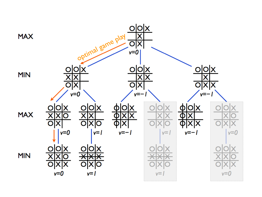
You should simulate the algorithm to see that the two branches that are grayed out indeed get pruned -- therefore, it is actually a bit misleading to even show their minimax values since the algorithm never computes them.
Remember that the Max nodes (such as the root node) only update
the alpha value and pass it down to the next
child node. Check that you reach a situation where
alpha=0 and beta=-1 in a
Min node. Actually you should reach such a situation twice.
Another good example (except for the choice of colors) can be found
from Bruce Rosen's lecture notes for Fundamentals of Artificial
Intelligence - CS161 at
UCLA: here.
Note in particular how he emphasizes the fact that the tree is only
expanded node by node as the algorithm runs, instead of running the
algorithm on a full tree as is often suggested by diagrams such as
the ones we use in this material (shame on us!). Rosen's example
also illustrates a scenario where the value of the game is not
constrained to be -1,0, or +1, and the algorithm starts at the root
with alpha = -∞ and
beta = ∞.
Maxine wants to try again -- best out of three! Minnie agrees and after a while, they arrive at the following position
       O|X|O
       -+-+-
       X| |X
       -+-+-
        |O|
It's again Min's turn to play an O. Evaluate the value of this state
of the game as well as the other states in the game tree where the
above position is the root, using alpha-beta pruning. Start the
recursion by calling min-value(root, -1, 1) where
root is the above board position.
What is the value of the game, and what are the optimal moves?
Notice that while the left-to-right order of the children of each node, i.e., the order in which the children are processed in the loop on lines 4--7, is arbitrary, it can have significant impact on which branches are pruned.
Now we feel confident enough about concepts and ideas behind the Minimax algorithm and alpha-beta pruning that we can start programming. We'll implement a tic-tac-toe bot.
- First implement the basic framework for the game: a data structure (class) for board positions, the functions for checking whether either player has a row of three, and a function for producing the list of children for a given board position.
- Then implement the Minimax algorithm according to the pseudo-code given above. The algorithm should return for any given board position, the value of the game: -1, 0, or 1.
- Using the previous step, modify the program so that it also outputs the optimal move for the player whose turn it is (which is given as an input, of course). You can do this by keeping record of the child node that yields the highest (lowest) value in a Max (Min) node.
- You can test the solution at this stage by using it to solve the above pencil-and-paper exercises.
- As the culmination of this exercise, modify the algorithm to
implement alpha-beta pruning as detailed in the pseudo-code
above. To see whether you gain any speed-up, you can see how
long the algorithm runs (or how many recursive function calls
are performed) with or without alpha-beta pruning -- simply
comment out line 7 with the test
alpha >= betato revert back to vanilla Minimax.
Reasoning under Uncertainty
In this section, we'll study methods that can cope with uncertainty. The history of AI has seen various competing approaches to handling uncertain and imprecise information: fuzzy logic, non-monotonic logic, the theory of plausible reasoning et cetera. In most cases, probability theory has turned out to be the most principled and consistent paradigm for reasoning under uncertainty.
If you want an objective and diplomatic view on the matter, don't ask me. I'll just repeat a counter-argument made by a proponent of fuzzy logic when he tried to get around a rigorous formal proof showing that any method of inference where degrees of plausibility are represented as real numbers, other than probability theory, is inconsistent: the response of the fuzzy logic proponent was that since the proof is based on ordinary (two-valued) logic, it doesn't apply to fuzzy logic. Now that is a counter-argument that is hard to refute!
Probability Fundamentals
We are working to add material about the basic concepts of probability theory: probabilistic model, events, joint probability, conditional probability, etc.
Since this section is not finished yet, feel free to refresh these concepts from your favorite source. Two great examples are:
- Ian Goodfellow, Yoshua Bengio & Aaron Courville: Deep Learning (Section 3)
- Charles Grinstead & J. Laurie Snell: Introduction to Probability
- Wikipedia: Bayes theorem (Section Drug testing)
- Youtube: Maths Doctor, A Level Statistics 1.5 Bayes' Theorem and medical testing
- Better Explained: Understanding Bayes Theorem with Ratios
The lecturer has two dice in his office (true story). One of them is an ordinary die and will yield any result from one to six with equal probability. However, the other die is loaded (true story, again). It will yield a six with probability 1/2 and any other outcome with probability 1/10. He will roll the ordinary die first, and then the loaded one. Calculate the following probabilities. Recall that P(A|B) means the conditional probability of A given B.
- P("both outcomes are 6")
- P("neither outcome is 6")
- P("the sum of the outcomes equals 9")
- P("the sum of the outcomes equals 9" | "at least one outcome is 6")
- P("at least one outcome is 6" | "the sum of the outcomes equals 9")
Hint: We know that probability calculus can be confusing, but keep calm and carry on, you'll get the hang of it!
Let's use the same dice as in the previous exercise.
- What is the distribution of the sum of the outcomes when rolling the ordinary die twice?
- What is the distribution of the sum of the outcomes when rolling the loaded die twice?
- Assume that either die (ordinary or loaded) is selected
at random with probability 1/2 each. The selected die is
rolled twice. Calculate the probability
P("the die is loaded" | "the sum of the outcomes is 10")
Calculate the probability that the die is ordinary as well to make sure that the sum of the two probabilities equals one. - Again, either die is selected with equal probability.
We notice that every time the die is rolled, the outcome is six.
After how many rolls can we be at least 99% sure that the
die is loaded?
Hint: Calculate the ratio of the posterior probabilities of each die after k rolls. If the posterior probability of the loaded die is over 99%, then the ratio of the posterior probabilities is over 0.99/0.01 = 99.
If you have trouble with these exercises, you may wish to study additional material on the Bayes rule. Good pointers are provided above.
An important announcement! Due to the great popularity of the course, we have been able to create a 4th exercise group. It's on Wednesdays at 2-4pm. The language will be English. We request that everyone who can, move to the new group. Especially those who are currently in group 99. Note that as this hopefully creates vacancy in the other groups, students currently in group 99 can choose any of the other groups in case there is space left.
From next week on, visiting another group will be allowed only if requested in advance. This also applies to those who may at that time still be registered to group 99.
It's time to say goodbye to the legendary 99.