Last week we practiced game algorithms, Minimax and alpha-beta pruning, on the simple game of tic-tac-toe. Tic-tac-toe is a good choice for understanding the basic principles and simulating the algorithms step-by-step. However, it is hardly a very cool AI application.
Now we'll change gears and go for what used to be thought as a some kind of a "grand challenge" for AI, namely chess! (In fact, that's not exactly true since we'll be playing a variant of chess, called Los Alamos chess which is played on a 6 x 6 board with no bishops.)
Implementing the complete game engine with all the rules is somewhat tedious, so we have done it for you. Also, since you've already implemented alpha-beta pruning last week, you don't have to do it again here. Instead, your task is to implement a heuristic evaluation function. The performance of the chess bot is in part determined by the goodness of the evaluation function, so designing a good one is critical for creating a competitive bot.
To make things exciting, we'll have a chess-bot tournament. You will submit your solution (the heuristic evaluation function) on our server and compete against our own contender, Deep Glue and bots by other students. May the best bot win!
- Download the Java template here. NB: There was an error (old version) in the package and it was fixed on Sept 21, 4.20pm. If you have problems uploading to the server, please reload the new package and try again.
-
Implement the method
double eval(Position p)in classYourEvaluator. The method takes as its input a board positionpwhich specifies the positions of all the pieces on the board and which player's turn it is. The return value should be the higher the more likely the white player is to win. -
You can upload the compiled
YourEvaluatorclass (i.e., theclassfile) on the tournament server. (If you use multiple classes, you can also upload a JAR file.) - Once you have uploaded your bot, you can play it against the other bots. You gain points by winning and lose points by losing. The highest ranked bot will be declared the champion at the end of the course. (One week before the exam.)
Probabilistic Inference
Let's now move ahead with the theme Reasoning under Uncertainty, and see how probability can be used for inference in various AI problems.
| Theme | Objectives (after the course, you ...) |
| Reasoning under uncertainty (continued from last week) |
|
Bayes rule and probabilistic inference
Bayes rule has a central role in statistical inference and machine learning. The basis for this is that it can be applied in scenarios where one of the random variables in the model corresponds to an unknown "state" which we are interested to learn. If the model includes other variables that correspond to "observations" that can be made and that are dependent on the unknown state, we can use the Bayes rule as follows
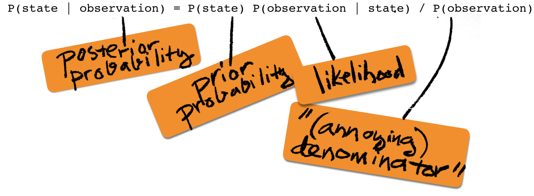
The left side of the equation is called the posterior probability (probability after the observation). The first factor on the right is called the prior probability (probability prior to the observation), the middle factor is called the likelihood (how likely the observation is when the state is given), and the last term on the right has many names, of which the annoying denominator may be the most fitting. (Evidence and marginal likelihood are more common.)
As you may have noticed, when completing last week's exercises, and as you will notice at the latest when completing this week's, calculating the denominator may indeed be annoying.
A nice trick that can sometimes save a lot of effort is to calculate the ratio of posterior probabilities, instead of the probabilities themselves. For example, consider the following ratio
R = P(State=1 | obs) / P(State=2 | obs)
where obs is an abbreviation for observation.
Applying Bayes rule to both the numerator and the denominator
in the ratio, we'll notice that the denominator P(obs)
cancels:
     P(State=1) P(obs | State=1) / P(obs)   P(State=1) P(obs | State=1)
R =  ------------------------------------ = ---------------------------
     P(State=2) P(obs | State=2) / P(obs)   P(State=2) P(obs | State=2)
In case the two states (1 and 2) are the only possibilities, we
have P(State=2|obs) = 1-P(State=1|obs) (because one of
the events must happen and both cannot occur at the same time).
In this case, after calculating the the above ratio, R,
it can be mapped back into the posterior probability of state 1 by
P(State=1 | obs) = R / (1+R)
You can check that this is true by assigning and using the
fact P(State=2|obs) = 1-P(State=1|obs).
Naive Bayes classification
One of the most useful applications of the Bayes rule is the so called naive Bayes classifier. It is a machine learning technique that can be used to classify objects such as text documents into two or more classes. The classifier is trained by analysing a set of training data, for which the correct classes are given.
The naive Bayes model is a probabilistic model that involves a class variable -- this corresponds to the state variable above -- and a number of feature variables. The assumption in the model is that the feature variables are conditionally independent given the class. (We will not discuss the exact meaning of conditional independence on this course. You can find more about it from the literature. For our purposes, it is enough to be able to exploit conditional independence in building the classifier.)
We will use a spam email filter as a running example for illustrating the idea of the naive Bayes classifier. Thus, the class variable indicates whether a message is spam (or "junk email") or whether it is a legitimate message (also called "ham"). The words in the message correspond to the feature variables, so that the number of feature variables in the model is determined by the length of the message.
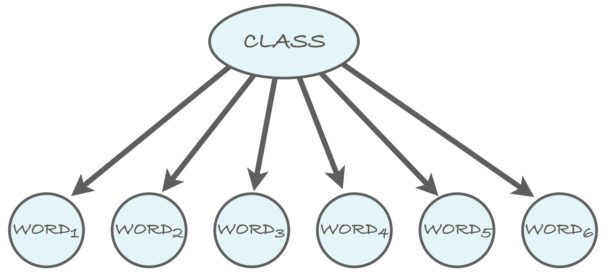
The naive Bayes model can be represented as a Bayesian network, which encodes the conditional independence between the feature variables (in this case, the words of the email message) given the class variable as in the above diagram. We'll return to Bayesian networks in the next section below.
Estimating parameters
To define the naive Bayes model, we need to specify the distribution
of each variable. For the class variable, this is the distribution
of spam vs ham messages, which we can for simplicity assume to be
1:1, i.e., P(spam) = P(ham) = 0.5.
For the feature variables, we will define two distributions: one for the spam messages and another one for the ham messages. In each case, we will make the simplifying assumption that each of the words in the message is distributed according to the same distribution. And as we said above, we also assume that the words are independent of each other given the spam/ham class.
The word distributions for the two classes are
best estimated from actual training data, i.e., a
corpus of spam messages and a corpus of legitimate messages. The
simplest way is to count how many times each word, aardvark,
aardwolf, ..., Zyzzogeton, appears in the corpus and dividing
the number by the total number of words in the corpus.
To illustrate the idea, let's assume that we have at our disposal both a spam corpus and a ham corpus. You can easily obtain one by saving a batch of your emails in two files.
Assume that we have calculated the number of occurrences of the following words in the two classes of messages:
        word    spam     ham
 ----------- ------- -------
 million         156      98
 dollars          29     119
 adclick          51       0
 conferences       0      12
 ----------- ------- -------
       total   95791  306438
One problem with estimating the probabilities directly from the counts is that the zero counts lead to zero estimates. This can be quite harmful for the performance of the classifier -- it easily leads to situations where the ratio of the posterior probabilities obtained as 0/0. That sounds dangerously close to the Singularity, so we'd better find a better way. The simplest solution is to use a small lower bound for all probability estimates. The value 0.000001, for instance, does the job.
We can now estimate that the probability that a word in a spam
message is million, for example, is about 156/95791
≈ 0.0016285. In other words, on the average, roughly every
614th word in a spam message is million. Likewise, we
get the estimate 0.0003198 for the probability that a word in a ham
message is million. Both of these probability estimates
are small but more importantly, the former is higher than the
latter. This turns out to be a sign that the word in question hints
towards the message being spam -- which sounds logical. Words for
which the ratio of the probabilities is the other way around, hint
towards the message being ham.
Classifying new data
After the parameters of the model have been estimated, the
classifier is ready for use! When we are given a new message, we
will compute the posterior probability P(spam |
message), where message is a place-holder for
the words in the message, for example, P(spam | 'million',
'conferences') (which would be a really short message).
Let's compute the posterior probability
P(spam | Word1 = 'million', Word2 = 'conferences')
which is abbreviated without a great risk of confusion -- but please
note that unlike million and conferences,
which are hyphenated ('like this') to indicate that they are words that occur
in the message, the term spam indicates
the class of the message, not the word "spam" -- as
P(spam | 'million',
  'conferences')
By Bayes rule, we have
                                      P(spam) P('million', 'conferences' | spam)
 P(spam | 'million', 'conferences') = ------------------------------------------
                                            P('million', 'conferences')
The numerator on the right side is the likelihood term and its meaning
is the probability that the first two words are million
and conferences given that the message is spam. The
denominator on the right side -- it's the annoying one -- is the
probability that the first two words are as stated when the spam/ham
status of the message is not given.
Let's look at the likelihood term first. The conditional independence assumption, i.e., the naive Bayes assumption, implies that the likelihood can be "factorized" as follows
P('million', 'conferences' | spam) = P('million' | spam) P('conferences' | spam)
This is very useful since these are the kind of probabilities we have estimated from the data. The same factorization rule can be applied no matter how many words there are in the message.
Next up is the annoying denominator. However, we'll use the hint above and avoid calculating the denominator (at least explicitly). To achieve this, we consider the ratio of posteriors:
 P(spam | 'million', 'conferences')   P(spam) P('million', 'conferences' | spam) / Z
 ---------------------------------- = ----------------------------------------------
  P(ham | 'million', 'conferences')    P(ham) P('million', 'conferences' | ham) / Z
where Z, defined as Z = P('million', 'conferences'),
is the annoying denominator which cancels out just as promised in the hint.
The term P('million', 'conferences' | ham) is treated in the exact
same manner as the term corresponding term for spam (see above), and the
numbers required to calculate its value are available since we have
estimated them from the training data.
The following exercises will demonstrate the use of the naive Bayes model.
Consider the word counts given in the table above (million, dollars, etc).
- Estimate the remaining word probabilities for both classes.
-
Use the obtained estimates to calculate the probability
P(Word ≠ 'million'), i.e., the probability that a single word in a message is notmillionwhen the class of the message is unknown. Hint: You should recall the rule for calculating the marginal probability (see, for example, the references given under Section 3.1 Probability Fundamentals of Part 2). -
Calculate
P(spam | 'million'), i.e., the probability that the message is spam given that its first word (or in fact, any particular word) ismillion. -
Calculate
P(spam | 'million', 'dollars', 'adclick', 'conferences'), i.e., the probability that the message is spam when its first four words are as stated.
Use the prior probability P(spam) = 0.5.
Additional hints: In item 3, remember Bayes. In item 4, remember to use a lower bound on the estimates. Also recall the trick about not calculating the annoying denominator.
Implementation details
The above exercise should make it relatively straightforward to see how the filter can be implemented by programming: the key insight is the routine nature of the word-by-word calculations.
A convenient way to group the computations is obtained by slight reshuffling of the terms. Consider still our example two-word message, and the following formula for the ratio of the posterior probabilities
     P(spam | 'million', 'conferences')
 R = ----------------------------------
      P(ham | 'million', 'conferences')

     P(spam) P('million' | spam) P('conferences' | spam)
   = ---------------------------------------------------
       P(ham) P('million' | ham) P('conferences' | ham)
Since the ratio of products is equal to the product of ratios -- i.e., for example, (ABC)/(DEF) = (A/D)(B/E)(C/F) -- we can group the above terms as
     P(spam)  P('million' | spam)  P('conferences' | spam)
 R = -------  -------------------  -----------------------
     P(ham)   P('million' | ham)   P('conferences' | ham)
More generally, the formula is
       P(spam)  N  P(word_i | spam)
   R = -------  Π  ----------------
       P(ham)  i=1 P(word_i | ham)
where N is the number of words in the message, and word_i is the
i'th word in the message.
Intuitively, the above formula encodes the rule that any word whose
probability is higher in spam messages than in ham messages will
increase the ratio R, and vice versa. For example, in our two-word
message, for i=1, we have word_i =
'million', and the ratio of the word probabilities is
given by
    P(word_1 | spam)   P('million' | spam)   0.0016285
    ---------------- = ------------------- ≈ --------- ≈ 5.1
    P(word_1 | ham)    P('million' | ham)    0.0003198
Thus, each occurrence of the word 'million' in the message
leads to roughly a five-fold increase in the posterior probability ratio.
Putting things together, here's a pseudocode sketch of the classification stage where we assume that the probability estimates have already been calculated from training data.
1:  spamicity(words, estimates):
2:     R = estimates.prior_spam / estimates.prior_ham
3:     for each w in words:
4:        R = R * estimates.spam_prob(w) / estimates.ham_prob(w)
5:     return R
Here estimates is an object that stores the estimated
probabilities: estimates.prior_spam is the probability that
a message is spam, P(spam), estimates.prior_ham the same
for ham; estimates.spam_prob(w) is the probability
P(Word = w | spam), and estimates.ham_prob(w)
the same for ham.
When dealing with long messages, the posterior probability ratio becomes a product with very many terms. This can easily lead to trouble because products are creatures that easily grow very very large or very very small (close to zero); the mathematical term is 'exponential rate'.
In order to reduce the risk of under- and overflows in the floating
point arithmetics, it is a good idea to carry out the computations
in log-scale. That is, instead of computing the ratio, R, you
should compute its logarithm, log(R). (Store the log-ratio in a variable
like logR.)
The important thing to recall about logarithms is that they convert multiplication into addition: log(AB) = log(A) + log(B); and similarly, division becomes subtraction: log(A/B) = log(A) – log(B). Using these, we can write the log-ratio as
                                       N
   logR = log(P(spam)) - log(P(ham)) + Σ [log(P(word_i | spam)) - log(P(word_i | ham))]
                                      i=1
The base of the logarithm (natural, 2, 10, ...) is not
consequential. The important thing is to map the end result back to
the ratio by exponentiating the log-ratio with the same base. So if
you use natural logarithms, for instance, then you should
exponentiate the log-ratio by exp(logR) to get R.
Next you get to implement a naive Bayes spam filter by
programming. The Java template is available on TMC. (In case you
prefer to use another programming language, feel free to. You can
find the ready-made spam and ham word count
files, spamcount.txt and hamcount.txt in
the template.)
-
Download the template and take a look at the word count files in
the template, which originally come from the development team of
the SpamAssassin
spam filter. The common "stop-words" that are uninteresting for
our present purpose, such as the, a, to, ... have been
removed, as have words that occur only once. The files are
sorted so that the most common words in the respective class
come first:
	top 10 spam words: top 10 ham words:
        ------------------ -----------------
         624 free          1776 list
         465 email         1263 lists
         414 money         1204 use
         410 please        1007 exmh
         410 mail           987 like
         383 list           952 some
         360 click          919 wrote
         358 content        909 linux
         339 business       895 listinfo
         306 information    893 rpm
The total number of unique words in the spam messages is 6245, and the total word count is 75268. The ham messages have 16207 unique words and the total word count is 290673. -
Estimate the conditional probabilities
P(Word=s | spam)andP(Word=s | ham)for all wordssthat occur in the files. For example, you should get the estimateP('free' | spam)≈ 0.00829. - Now implement a filter that reads a new message and calculates the probability that it is spam using the naive Bayes model, following the instructions above.
-
Test your classifiers by running it on the two example messages that come with
the TMC template
spamesim.txt(which should classified as spam) andhamesim.txt(which should be classified as ham). You can also try your spam filter on your own email messages.
Hint: In item 3, you may encounter words that you haven't encountered in the training data at all. You can use the small constant lower bound for them.
Here is some additional material on naive Bayes spam filtering that you may like to take a look at:
- Dr Dobbs Journal: Naive Bayesian text classification
- M. Sahami, S. Dumais, D. Heckerman, E. Horvitz (1998). "A Bayesian approach to filtering junk e-mail". AAAI'98 Workshop on Learning for Text Categorization.
Bayesian networks
As we mentioned above, the naive Bayes model is a kind of a Bayesian network, with an associated graph structure where the class variable is the root and the only "parent" of all the feature variables.
Bayesian networks are a model family which belong to the still more general category of (probabilistic) graphical models, which are a modeling "language" for probabilistic models. The power of graphical models is mainly due to i) their ability to compactly represent multivariate domains with complex dependencies, and ii) efficient inference procedures that exploit the structure of the models.
Building blocks of a Bayesian network
A Bayesian network will represent a joint distribution over a number of random variables. Depending on the complexity of the network (which depends on the number of placement of the edges in the graph), the Bayesian network representation may require significantly fewer numerical parameters than the number of elementary events in the domain.
The structure of the network is encoded as a graph where each random variable is represented as a node, and the dependency structure is characterized by a set of directed edges between the nodes. The graph must be a directed acyclic graph (DAG), which means that it is impossible to start from a node follow a path in the direction of the edges to arrive at the same node.
Here's an example DAG:
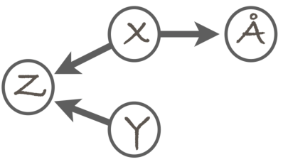
The random variables in the model are X,Y,Z, and Å. (For the non-Scandi students, the last one is what we call the "Swedish O" in Finland; see Wikipedia:Å. It conveniently comes after X, Y, and Z in our alphabet.) The edges correspond to direct dependency, so that the absence of an edge between any two variables means that the variables are conditionally independent given some (possibly empty) set of other variables. The details of this are slightly too complicated to discuss here, so we'll not go into them. For now, it is enough to remember that the edges are a way to encode the dependency structure in the domain.
In addition to the structure encoded as the DAG, a Bayesian network comes with a set of parameters quantifying the conditional distributions of the variables. These are given in the form P(V=v | PaV = paV), where V is a random variable and v is a value, and PaV denotes the parents of node V in the graph: i.e., the nodes from which there is an edge to V. For example, in the above DAG, we have PaZ = {X,Y}, and PaY = ∅ because node Y has no parents at all.
When the variables are categorical, i.e., they take values in a finite set, the conditional distributions can be specified as conditional probability tables (CPTs). A CPT for variable V includes the distribution of V for each possible combination of the values of V's parents. We call such combinations parent configurations. For example, if in the above example network, all variables are binary, then the parent configurations of Z are (X=0, Y=0), (X=0, Y=1), (X=1, Y=0), (X=1, Y=1), and the CPT of Z will have four rows, each containing a conditional distribution for Z. A concrete example is as follows
| Z | |||
| X | Y | 0 | 1 |
| 0 | 0 | 0.1 | 0.9 |
| 0 | 1 | 0.2 | 0.8 |
| 1 | 0 | 0.5 | 0.5 |
| 1 | 1 | 0.0 | 1.0 |
So for instance, if X=1 and Y=0, then the conditional probability of Z=1 is given by P(Z=1 | X=1, Y=0) = 0.5, and so on.
For a variable that has no parents in the network, the CPT is actually just a single distribution, and the CPT has only one row. For variables that have many parents, the CPT may easily become very very large.
To make things concrete, we use a running example which is the
car Bayesian network discussed at the lecture. Its structure is
the following:
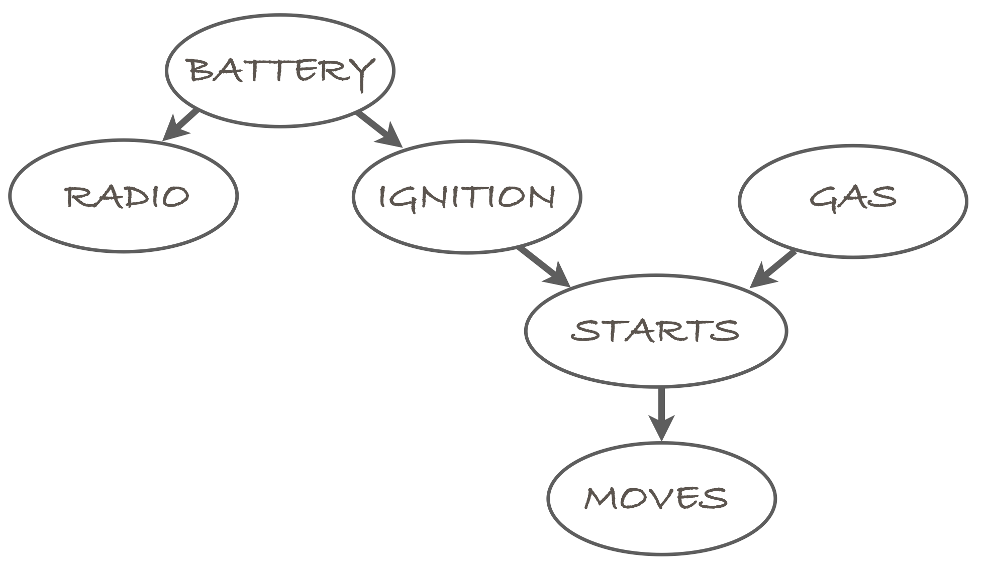
The variables in the model are abbreviated as the first letters:
    [B]attery
    [R]adio
    [I]gnition
    [G]as
    [S]tarts
    [M]oves
The CPTs are as follows:
| B | |
| 0 | 1 |
| 0.1 | 0.9 |
| R | ||
| B | 0 | 1 |
| 0 | 1.0 | 0.0 |
| 1 | 0.1 | 0.9 |
| I | ||
| B | 0 | 1 |
| 0 | 1.0 | 0.0 |
| 1 | 0.05 | 0.95 |
| G | |
| 0 | 1 |
| 0.05 | 0.95 |
| S | |||
| I | G | 0 | 1 |
| 0 | 0 | 1.0 | 0.0 |
| 0 | 1 | 1.0 | 0.0 |
| 1 | 0 | 1.0 | 0.0 |
| 1 | 1 | 0.01 | 0.99 |
| M | ||
| S | 0 | 1 |
| 0 | 1.0 | 0.0 |
| 1 | 0.01 | 0.99 |
Just to take an example, the car will start (S=1) with probability 0.99 in case the ignition works (I=1) and there is gasoline in the tank (G=1). (No Tesla obviously). If there's a problem either with the ignition or the gasoline, then the car won't start for sure, i.e., P(S=1 | I=i, G=g) = 0.0 for all other combinations (i,g) than (1,1).
The structure (the DAG) and the parameters in the CPTs are the building blocks of a Bayesian network. Next we dicuss how they represent a joint distribution and how they can be used to perform inference about the domain.
Defining a probabilistic model as a Bayesian network
A probabilistic model is really nothing but a joint distribution over the random variables in the domain. The joint distribution defines the probability of each elementary event, which are equivalent to joint value assignments for the random variables. In the car domain, an elementary event is defined by six bits, B,R,I,G,S,M. For example, the event 1,1,1,1,1,1 would be a good day: the battery is alive, you listen to some good music, the car starts because you remembered to fill the tank yesterday, and you make it to the lecture in time.
The joint probability of any elementary event is obtained as the
product of the conditional probabilities of the form P(V=v |
PaV = paV), where you'll recall PaV
refers to the parent set of V. In the car domain, the product is
thus of the form:
P(B=b,R=r,I=i,G=g,S=s,M=m) =
P(B=b) P(R=r | B=b) P(I=i | B=b) P(G=g) P (S=s | I=i,G=g) P(M=m | S=s),
where b,r,i,g,s, and m denote values of the respective random
variables. The above formula is called a factorization
of the joint probability.
To make it easier to interpret the events we won't use the rather long notation like B=1,R=1,I=1,G=1,S=1,M=1 or even the shorter notation like 1,1,1,1,1,1 to denote events in the car domain. Rather, we'll have a different label for the values of each of the random variables. For the variable Battery, we denote the good case (battery is alive) by B and the bad case by ¬B. Similarly, for Radio, we denote the good case (music is played) by R, and the bad case by ¬R, and so on.
This is actually slight abuse of notation since we also denote the corresponding variables by the initial letters, B, R, etc, but we hope the meaning is clear enough.
The probability of a good day with the car is
P(B) P(R|B) P(I|B) P(G) P(S|I,G) P(M|S)
= 0.9 × 0.9 × 0.95 × 0.95 × 0.99 × 99
≈ 0.716.
Pay close attention to the form of the terms, and make sure you could
choose the right values from the above CPTs to do the above
calculation.
Or, some days are fine except the radio may not work, which is
denoted as ¬R. The probability of the elementary event where
everything else is good but the radio is out is obtained similarly,
and the result is:
P(B) P(¬R|B) P(I|B) P(G) P(S|I,G) P(M|S)
≈ 0.080.
Check that you get the same result by substituting the numbers from
the CPTs in the correct places. Remember that ¬R means R=0 (see the
hint above).
You may ask what the point in all this business with the CPTs is: having to come up with all the numbers (parameters) in the CPTs looks like a lot of work. Why not just directly try to come up with the probabilities of the elementary events if that is the end result? The answer is that we can sometimes save a whole lot of work this way. In the car example, the CPTs contain 2+4+4+2+8+4 = 24 numbers, of which half are actually redundant since the numbers on each row must always sum up to one, i.e., there are really only 12 numbers to choose. The number of elementary events, on the other hand, is 26=64, i.e., we would have to come up with 63 parameters (the last one could be obtained by subtracting the others from 1.0). This shows how Bayesian networks can lead to compact representation of probabilistic models.
Exact inference in Bayesian networks
Compact representation of probabilistic models is only one of the two main advantages of Bayesian networks. The other advantage is efficient inference. Here we will discuss what we mean by inference, but to get to the efficient inference algorithms, you will have to study a bit more than this course.
Just like in the above examples where we used Bayes rule and other probability calculus methods to compute posterior probabilities of the kind P(state | observations), we can do the same with Bayesian networks. Continuing with the car example, we can for example compute P(battery dead | radio doesn't work, car won't move), or P(¬B | ¬R, ¬M), to figure out what is wrong with our car.
So, let's get to work. We can start by writing the conditional probability as a ratio of two probabilities
                   P(¬B, ¬R, ¬M)
  P(¬B | ¬R, ¬M) = -------------
                      P(¬R, ¬M)
To obtain these probabilities, we need to use the marginalization
rule, which we have used before to write the annoying denominator
as a sum of two terms. Here the sum will be composed of many
terms instead of only two, but the basic principle is the same.
The numerator becomes:P(¬B, ¬R, ¬M) = Σω ∈ (¬B,¬R,¬M) P(ω)
= P(¬B, ¬R, I, G, S, ¬M)
+ P(¬B, ¬R, I, G, ¬S, ¬M)
+ P(¬B, ¬R, I, ¬G, S, ¬M)
+ P(¬B, ¬R, I, ¬G, ¬S, ¬M)
+ P(¬B, ¬R, ¬I, G, S, ¬M)
+ P(¬B, ¬R, ¬I, G, ¬S, ¬M)
+ P(¬B, ¬R, ¬I, ¬G, S, ¬M)
+ P(¬B, ¬R, ¬I, ¬G, ¬S, ¬M)
where ω ∈ (¬B,¬R,¬M) denotes the set of elementary events that belong to the event (¬B,¬R,¬M).
We can now obtain the probability of each of the above eight
elementary events by using the factorization into a product of
conditional probabilities, and substituting the appropriate values
into the product from the CPTs. Take the first one:
P(¬B, ¬R, I, G, S, ¬M)
= 0.1 × 1.0 × 0.0 × 0.95 × 0.0 × 1.0 = 0.0
which turns out to be equal to zero. Can you see why this makes sense?
(Remember the meaning of ¬B and I. Can they happen at the same
time?)
The denominator in the formula for the posterior probability we wish to compute, P(¬R, ¬M), can also be evaluated using the same technique. It will involve a sum of 16 terms since there are four variables that we need to sum over when we expand the event into a sum of elementary events. But if we work hard and do the math, we'll get the answer we need.
We call this the brute-force approach, and it has the advantage that it always leads to exactly the right answer. Implementing the calculations in a computer avoids the tedious task of writing down large sums and manually calculating them. However, in larger domains than our small car example, the calculations will become infeasible even for a computer. The problem is that the number of terms to be evaluated grows exponentially with respect to the number of variables in the model. That is why the more advanced and efficient inference algorithms that we've alluded to a few times are such an important thing. Another solution is to use approximate inference, which is our next topic.
Generating data from a Bayesian network
In order to do approximate inference, we need to be able to generate (or sample) data from the joint distribution defined by a Bayesian network. The data will consist of tuples, each of which is essentially a list of values for each of the random variables in the domain. Thus, each tuple corresponds one-to-one to an elementary event ω.
The algorithm to generate tuples is quite simple. We first choose values for any variables that have no parents. The choice is done randomly according to the distribution defined by the CPT. For example, to choose the value for the Battery variable in the car model, we use the distribution (0.1, 0.9). Similarly, the value of variable Gas is drawn from the distribution (0.05, 0.95).
You have probably generated numbers from a pseudorandom number
generator in your favorite programming language. In python, you may
have used random.random(), and in Java, Math.random().
Both of these return pseudorandom floating point values in the range
[0.0, 1.0). Other functions exist for generating random integers,
Booleans, etc.
Some languages also have functions to generate categorical values (values in a finite set) from a given distribution. If your favorite language doesn't provide such functions, it is easy to apply the existing functions to implement them.
For binary variables, the method works as follows. Let the
probability of zero in the distribution you wish to sample from be
some P(X=0). Generate a random floating point value r
by the aforementioned functions. If r < P(X=0), then
output the value 0, and otherwise 1. Clearly a uniformly distributed
value between 0 and 1 is less than P(X=0) with probability P(X=0), so
our method produces value 0 with probability P(X=0), as it should.
In the following, we will only need the binary case, but just in
case you are interested: For categorical variables with more than
two values, the method works in a similar fashion. The value 0 is
produced if r is less than P(X=0). The value 1 is
produced if r is between P(X=0) and P(X=0)+P(X=1). And
generally, the value x is produced if
r is between A = Σi=0,...,x-1 P(X=i)
= P(X=0) + ... + P(X=i-1) and A + P(X=i).
To choose values for the remaining variables, we proceed in such an order that when dealing with a variable, we have already chosen the value(s) for its parent(s). After choosing the value for Battery, we can thus move on to variable Radio. The distribution from which we choose the value of a child variable (such as Radio) is determined by the configuration of its parents (such as Battery). If B=1, then we draw the value of R from distribution (0.1, 0.9). Whereas if B=0, then we draw the value of R from distribution (1.0, 0.0) and the outcome is always R=0. No battery, no music.
Note that when choosing the value of Starts, we need to chosen the values of both Ignition and Gas.
Pseudocode for a generating n random tuples from a Bayesian network is as follows.
1: generate_tuples(n, model):
2:
   for i = 1 to n:
3:       v = empty array
4:       for V in model.variables:
5:          pa = v[V.Pa]    # parents of V
6:          v.append(sample(V.CPT(pa)))
7:       output v
In the pseudocode, model is an object that defines the
Bayesian network model by giving for each variable V a
set of parents (in the form of a set of indices that can be used to
select variables in array v), and the corresponding
CPTs. The selection operator v[V.Pa] extracts from the
array the elements that define the values of the parents
of V. These are used on line 6 to choose the correct
row from the CPT of V. Note that here it is important
that the variables be processed in such an order that the parent
values are added into the array before they are needed for
generating the children.
Approximate inference (Monte Carlo)
The simplest approximate inference method is based on using the tuples sampled from a Bayesian network to estimate probilities directly as relative frequencies. To estimate the probability of an event, we simply draw a large number n of tuples, and count in how many of them the event occurs. The number of occurrences divided by n is then an estimate of the probability of the event.
Thus, we get
                    #{tuples where B=0, R=0, M=0}
    P(¬B, ¬R, ¬M) ≈ -----------------------------
                                  n
To approximate conditional probabilities, we simply write them as ratios, P(A | B) = P(A, B) / (B), and apply the same estimator to both the numerator and the denominator.
This is a very simple and general technique, which belongs to the category of Monte Carlo techniques due to the use of chance in obtaining the results. The downside is that the result is not exact. The variance that is caused by the random nature of the process can sometimes make the obtained probabilities quite inaccurate. The bigger the number of tuples, however, the better the accuracy, and in the limit as n → ∞ the approximation converges to the exact value.