Philosophy, problem solving as search, games
- Episode 1 (We 28/10, 2:15–4:00 PM): Course organization & what is AI and its philosophy? (Giulio)
- Episode 2 (Fr 30/10, 10:15 AM–12:00 PM): Search and problem-solving, Games (Indrė)
| Theme | Objectives (after the course, you ...) |
| Philosophy and history of AI |
|
| Games and search |
|
What is AI?
Artificial intelligence is not defined by one universally accepted sentence. It is a field of research and engineering whose boundaries move as technologies become familiar. Search, optical character recognition and speech recognition were once emblematic AI problems; when they became reliable, they increasingly came to be treated as ordinary computing infrastructure. This is sometimes called the AI effect.
It is therefore useful to distinguish an operational definition, which tells us what systems fall within a technical or regulatory scope, from a philosophical definition, which asks what intelligence, understanding or mind actually are. The first can guide engineering and governance without settling the second.
The updated OECD definition and the EU AI Act describe an AI system as a machine-based system that operates with varying levels of autonomy and may adapt after deployment. For explicit or implicit objectives, it infers from its inputs how to generate outputs such as predictions, content, recommendations or decisions that can influence physical or virtual environments.
The important words are machine-based, objectives, inference, outputs and influence. The definition does not require the system to resemble a human, be conscious, or use one particular technique such as machine learning.
Model, system and application
An AI model is a learned or programmed mathematical structure that transforms inputs into outputs. An AI system includes the model together with interfaces, data flows, tools, rules, monitoring, people and a context of use. For example, a language model is not by itself a clinical triage system. The latter also includes the user interface, patient data, prompts, retrieval tools, escalation procedures and human responsibility. This distinction matters because capabilities belong partly to models, while consequences and accountability arise from systems in use.
Four ways of asking whether a system is intelligent
Russell and Norvig organize influential approaches to AI around two distinctions:
| Human standard | Rational standard | |
|---|---|---|
| Thinking | Thinking humanly: does the system reproduce human cognitive processes? | Thinking rationally: does it draw correct conclusions? |
| Acting | Acting humanly: is its behaviour indistinguishable from human behaviour? | Acting rationally: does it choose actions expected to achieve its objectives? |
These approaches select different evidence. A system can act successfully without thinking like a human. A system can reason correctly in a simplified model and still fail in the world. Modern AI courses often use the rational-agent perspective: an agent receives information from an environment and selects actions according to a performance measure, given limited information, computation and time. This is a useful engineering stance, not a complete theory of human intelligence.
Narrow AI, general-purpose models and AGI
| Term | Useful meaning | Example or qualification |
|---|---|---|
| Narrow AI | A system with strong capabilities in a bounded task or domain. | A chess engine, spam filter or medical-image classifier. |
| General-purpose AI model | A model displaying significant generality and capable of performing a wide range of distinct tasks or supporting many downstream applications. | This is a legal category in the EU AI Act; it does not mean that the model possesses general intelligence. |
| Artificial general intelligence (AGI) | A contested research concept referring to broad and high-level competence across tasks and contexts. | There is no agreed scientific test or legal definition. |
Discussions of AGI often become confused because several different properties are compressed into one label. A clearer approach is to ask separately about breadth, performance, transfer, robustness, learning and autonomy. The Levels of AGI framework, for example, classifies systems using the breadth and depth of their capabilities while treating autonomy as a separate deployment dimension.
- AGI is not the same as consciousness: broad task performance does not establish subjective experience.
- AGI is not the same as autonomy: a capable model may be deployed with little independent control, and a simple system may operate autonomously.
- AGI is not the same as superintelligence: generality concerns breadth; superintelligence implies performance far beyond humans.
- AGI need not reproduce human cognition: similar performance can arise from very different mechanisms.
- AGI does not automatically imply moral status: that requires a further ethical and philosophical argument.
What would count as evidence for AGI?
A benchmark samples behaviour under specified conditions; it does not measure an entire mind. Strong scores can be influenced by training-data contamination, prompt design, tool access and evaluation choices. Real-world competence additionally requires reliability, recovery from errors, sensitivity to context and the ability to cope with consequences over time. When evaluating an AGI claim, ask:
- How broad are the tasks, and are genuinely novel tasks included?
- Is performance reliable or based on occasional successful demonstrations?
- Does knowledge transfer when the setting, representation or goal changes?
- Can the system recognize uncertainty and seek clarification or help?
- How much scaffolding is provided by prompts, humans, retrieval systems or tools?
- Is autonomy being measured separately from capability?
A brief history of AI: origins, optimism and setbacks
AI developed alongside computer science. Alan Turing's work connected the idea of mechanical computation with questions about intelligent behaviour. John McCarthy, Marvin Minsky, Nathaniel Rochester and Claude Shannon used the term artificial intelligence in their 1955 proposal for the Dartmouth summer research project, held in 1956. Its ambition was that aspects of learning and intelligence could be described precisely enough for a machine to simulate them.
Games, theorem proving and puzzles provided early testbeds: their states, legal moves and goals could be specified explicitly. Search and planning produced important advances, including methods related to the A* search and alpha-beta pruning studied in this course. Success in these restricted settings encouraged optimism about much broader machine intelligence, but moving from a well-defined problem to an open, changing world proved much harder.
Good Old-Fashioned AI (GOFAI) versus modern AI
GOFAI refers to the classical symbolic approach: represent knowledge as explicit symbols, facts and rules, then manipulate those representations through logical inference, search or planning. For example, an expert system might combine rules elicited from specialists to derive a recommendation. The difficulty is not only executing the rules: someone must identify relevant knowledge, encode it and keep it up to date.
The earlier course material used modern AI to emphasize methods that cope with uncertain, incomplete and noisy information. Probabilistic models represent degrees of uncertainty and update beliefs as evidence arrives. Machine learning estimates patterns or model parameters from data; deep learning also learns useful internal representations. These are related developments, but reasoning under uncertainty and learning from data are different capabilities: a probabilistic model can be specified by an expert, and a learned model need not explicitly represent uncertainty.
| Question | Classical symbolic AI / GOFAI | Probabilistic and learning-based approaches |
|---|---|---|
| How is knowledge represented? | Explicit symbols, facts, relations and rules. | Probability distributions, statistical models or learned representations. |
| Where does knowledge come from? | Mainly from people encoding a domain and its rules. | From expert assumptions, data, or a combination of both. |
| How are conclusions produced? | Inference, search and planning over explicit representations. | Probabilistic inference or predictions from learned models. |
| What works well? | Clearly specified constraints, structured problems and inspectable reasoning steps. | Noisy observations, pattern recognition and tasks where writing every rule is impractical. |
| What can go wrong? | Brittleness, missing knowledge, expensive maintenance and large search spaces. | Biased or inadequate data, distribution shift, uncertain reliability and difficult explanations. |
Example: identifying spam. A symbolic filter could apply a rule such as “if a message contains a particular phrase and comes from a blocked sender, flag it.” A learned classifier instead estimates patterns from labelled messages; a probabilistic classifier can estimate the probability of spam given the observed words. The first approach depends on the coverage of its rules; the second depends on the quality of its data and how well those patterns transfer to new messages.
This contrast describes broad emphases, rather than two mutually exclusive eras. Neural learning already existed in the early decades of AI, symbolic methods remain useful today, and systems can combine learned perception with explicit rules, search or planning. “Modern” does not mean that a system understands the world or will necessarily generalize reliably.
AI winters: when expectations exceeded results
An AI winter is a period of reduced funding, commercial investment and confidence in AI after expectations are disappointed. It does not mean that research stopped. Dates vary across accounts and countries, but two broad periods are commonly distinguished.
The first AI winter: roughly the mid-1970s to the early 1980s
Early demonstrations had encouraged claims that general machine intelligence was close. In practice, programs struggled with real-world language, perception and the rapid growth of search spaces. Computing resources and available data were limited. Criticism of simple perceptrons also weakened confidence in neural-network research, although the limitations of those models were not a proof that all neural networks were incapable. The 1973 Lighthill Report criticized progress in the UK, and changes in funding priorities in the UK and US contributed to a broader loss of support.
The second AI winter: roughly the late 1980s to the mid-1990s
The commercial expansion of expert systems brought renewed optimism. Some systems were useful in bounded domains, but acquiring and maintaining their knowledge was expensive, and they often struggled with unfamiliar situations. Disappointing returns, together with the collapse of the specialized Lisp-machine market as general-purpose computers became competitive, undermined investment. These problems concern the limits of particular technologies and business expectations; they do not imply that every expert system failed or that symbolic reasoning became useless.
Renewed growth: probability, data and learned representations
From the late 1980s and through the 1990s, probabilistic reasoning and statistical machine learning gained influence. Larger datasets, improved algorithms and increased computing power later supported the resurgence of neural networks as deep learning. Large pretrained models subsequently enabled reuse across many tasks and modalities. These developments overlap: they are not a single invention that suddenly ended a winter.
Success on a restricted task does not establish general intelligence. Ask what a system demonstrates, under which conditions it works, what resources it needs and whether claims go beyond the evidence. The history of AI connects directly to our philosophical questions: successful behaviour alone does not settle understanding, consciousness or the nature of human skill.
Connection to the course: Week 1 introduces search and games; Week 2 develops reasoning under uncertainty with probability and Bayesian methods. Later weeks explore learning and neural networks. The aim is to understand what each approach contributes and how they can be combined. For further historical context, see Russell and Norvig, the introduction to Artificial Intelligence: A Modern Approach.
On the philosophy of AI
Philosophy helps separate questions that are easily conflated. Behaviour asks what a system can do. Mechanism asks how it produces that behaviour. Understanding asks whether its symbols or outputs have meaning for the system. Phenomenology asks whether the system has subjective experience. Evidence bearing on one question does not automatically settle the others.
Turing: operationalizing intelligent behaviour
In Computing Machinery and Intelligence (1950), Alan Turing proposed an imitation game. A human interrogator exchanges written messages with hidden participants and attempts to determine which is human and which is a machine. Turing's move was methodological: rather than first defining an invisible inner property called thinking, examine observable linguistic performance. Passing such a test would be significant evidence of conversational competence, but it would not by itself explain the mechanism, establish consciousness or prove that the machine thinks in the way humans do.
Searle: syntax is not automatically semantics
John Searle's Chinese Room thought experiment asks us to imagine a person who does not understand Chinese but follows a rulebook for transforming Chinese symbols. To people outside the room, the answers may appear fluent and appropriate. Searle argues that formal symbol manipulation—syntax—is not by itself sufficient for meaning or semantics. The argument targets the claim that running the right program is sufficient for understanding; it does not show that AI systems cannot be useful or behave intelligently. Replies include the systems reply, robot reply and brain- simulator reply, each locating understanding in a larger system than the person following the rulebook.
Dreyfus: intelligence is more than rule-following
Hubert Dreyfus criticized a picture of intelligence that dominated much early symbolic AI: the world is first represented as explicit facts, cognition applies formal rules to those facts, and action follows from the resulting representation. His challenge was not simply that computers were too slow. It was that everyday intelligent activity depends on a background of embodied skills, habits, social practices and sensitivity to context that is not normally represented as an exhaustive list of facts and rules.
This argument draws on phenomenology, especially Heidegger and Merleau-Ponty. We are usually not detached spectators constructing a complete internal description of the world. We are already involved in meaningful situations: a door is encountered as something to open, a sentence as inviting a reply, and a changing traffic scene as calling for slowing down. Dreyfus called this practical, action-oriented engagement absorbed or embodied coping.
Knowing-that and knowing-how
Knowing-that is propositional knowledge that can often be stated explicitly: knowing that braking distance increases on an icy road. Knowing-how is skilled performance: feeling a loss of traction and adjusting appropriately before completing a conscious calculation. The distinction is not between reason and emotion, nor does it imply that experts never reflect. It means that competent performance is not exhausted by following explicit instructions.
The Dreyfus model of skill acquisition
Stuart and Hubert Dreyfus proposed that learners commonly move from reliance on context-free rules toward increasingly situated perception and action. The model is a philosophical and educational account, not a law that every learner follows identically.
| Stage | How the situation is encountered | Typical mode of action |
|---|---|---|
| Novice | Recognizes context-free features taught by an instructor. | Follows explicit rules. |
| Advanced beginner | Begins noticing recurring situational cues. | Combines rules with examples from experience. |
| Competent | Selects what matters from many possible features. | Plans deliberately and accepts responsibility for choices. |
| Proficient | Perceives the situation more holistically. | Sees what needs attention, while still deliberating about action. |
| Expert | The situation immediately appears in terms of meaningful possibilities for action. | Usually responds fluently and intuitively, while retaining the capacity to reflect when needed. |
Consider learning to drive. A novice may apply separate rules about speed, mirrors and distance. An experienced driver sees a wet road, a pedestrian's posture, a hidden junction and the rhythm of traffic as one meaningful situation. The relevant response is not produced by consciously enumerating every fact. Experience has changed what the driver notices and how the situation solicits action.
Dreyfus was right that brittle, hand-written rule systems do not scale gracefully to open environments and that relevance is difficult to specify in advance. However, his strongest predictions about what machines could never do were weakened by systems that learn patterns and representations from data. Chess, vision, speech and language systems achieved levels of performance that earlier symbolic programs did not.
Yet success without hand-written rules does not dissolve the philosophical problem. A learned model can be highly capable while questions remain about grounding, embodied experience, social practices, robust transfer and whether machine competence is the same kind of skill as human expertise. Neural learning changes the engineering premise; it does not automatically establish understanding or lived involvement in a meaningful world.
A working definition for this course
In this course, we use AI to refer to the study and construction of machine-based systems that perceive or receive information, infer or learn, and act or generate outputs in pursuit of objectives. This definition is broad enough to include search, probabilistic reasoning, machine learning, neural networks, language models, agents and robotics. It remains deliberately neutral about whether such systems possess consciousness or human- like understanding.
Keep the following distinctions in view throughout the course:
- an AI model is not the same thing as an AI system in use;
- general-purpose does not automatically mean general intelligence;
- successful performance does not by itself settle understanding;
- autonomy is not the same thing as consciousness;
- explicit rules are useful, but they may not exhaust human skill.
Selected sources
- OECD (2024), Explanatory memorandum on the updated definition of an AI system.
- European Union (2024), Artificial Intelligence Act, Regulation (EU) 2024/1689.
- Morris et al. (2024), Levels of AGI for Operationalizing Progress on the Path to AGI.
- Alan Turing (1950), Computing Machinery and Intelligence.
- John Searle (1980), Minds, Brains, and Programs.
- Hubert Dreyfus (1972/1992), What Computers Can't Do / What Computers Still Can't Do.
- Stuart E. Dreyfus and Hubert L. Dreyfus (1980), A Five-Stage Model of the Mental Activities Involved in Directed Skill Acquisition.
- Stuart Russell and Peter Norvig, Artificial Intelligence: A Modern Approach.
Your first exercise will be to take a look into current AI research. Find an AI-related scientific article from recent years. Pick one that you can understand, by and large: try to see what the problem statement, methodology, and conclusions are, roughly.
Good places to start your search are, e.g., the proceedings of AAAI, IJCAI, and ECAI conferences or magazine-style publications that may be somewhat less technical and intended for broader audiences, such as AI Magazine. However, please try to avoid articles that are overly polemic and superficial -- the idea is to take a look at academic AI, and ignore the BS on my Facebook feed...
Read the article through and answer the following questions:
- What is the research problem?
- Is the topic related to the topics of this course?
- Generally speaking, what impression does the article give about modern AI research? Reflect on the history and philosophy of AI discussed above.
- What studies would be needed to undertand the article in detail?
- Bonus question: Considering the article you chose, how relevant is the ''Terminator'' scenario where AI becomes self-conscious and turns against the humankind?
Most of the articles tend to be quite technical and focused on a narrow sub-problem.
The technical background required often includes maths such as formal logic and probability calculus, and computer science topics such as algorithms and data structures.
To take a concrete example, we can take a look at the article Polynomial Optimization Methods for Matrix Factorization by P.-W. Wang, C.-L. Li, and J.Z. Kolter, which appeared in the AAAI-17 conference.
- The article presents new algorithms for factorizing matrices (representing big matrices as products of smaller matrices) that are based on certain optimization techniques. Matrix factorization can be used in various machine learning scenarios. For example, many state-of-the-art recommender systems that predict user ratings of items such as movies or music include matrix factorization as a key component. Improving matrix factorization algorithms will thus eventually lead to better movie and music recommendations.
- The article is clearly relevant to the course topics (machine learning and recommendation systems in particular).
- Based on this article alone, AI research would appear to differ only slightly from mathematics research. The emphasis on practical solutions and empirical evaluation is a feature characteristic to AI and ML research.
- The paper uses advanced multivariate calculus tools. From an algorithmic point of view, there is actually nothing intricate (basically a few loops), and the maths background is the area where further studies would be required to get the details.
- The article doesn't mention consciousness or any other "philosophical" issues at all. The problem is clearly constrained as that of minimizing a function. The progress in AI that this paper makes is quantitative, not qualitative.
Solving the above exercise gives you one point (1p). Some exercises require a bit more effort, and they may give you two points (2p). This is indicated in the exercise heading as above.
Solutions to ''pencil-and-paper'' exercises such as this one are returned at the exercise sessions where you should make sure to mark completed exercises on the sheet that is circulated in the beginning.
Programming exercises come with a downloadable package that includes starter code and local tests. Download the package, implement your solution, and run the tests on your computer. Programming exercises are also marked at the exercise session.
We will now put our wine glasses aside, roll our sleeves, and turn our minds toward more practical considerations. Let's jump to our first technical topic: search and problem-solving.
Search and Problem-Solving
Many problems can be phrased as search problems. Formulating the search space and choosing an appropriate search algorithm often requires careful thinking and is an important skill for an AI developer.
Basic tree and network traversal algorithms belong to the course prerequisites, and you should already be familiar with breadth-first, depth-first, and best-first search (including its special case, the A* algorithm). If you forgot the details right after taking the exam, no need to worry: we will revisit them below.
Formulating Problems as Search
Being able to solve AI problems by search requires that we first formula the problem in a certain way.
The key concepts are the set of allowed states, called the search space, and transitions between them. Sometimes different transitions have different costs associated with them: think, for example, a tram or air travel network where the distances between two stops or airports are different. The cost can be sometimes measured in kilometers, sometimes in hours and minutes, and sometimes in some other resources.
The state transition diagram is a diagram where each allowed state is a node and the allowed transitions between them are shown as edges connecting the nodes.
The state transition diagram idea can be illustrated by the classic Wolf, Goat, and Cabbage puzzle. The puzzle involves a farmer who has (for some strange reason) a wolf, a goat, and cabbage. The farmer is transporting them across a river in a small boat that can only carry one piece of cargo at a time. However, the farmer can't leave the wolf alone with the goat, because when unattended, the wolf east the goat. Likewise, the goat can't be left alone with the cabbage for the same reason.
Feel free to first try to solve the puzzle using just your wit. You may have to think for a while before you figure it out!
We can represent each state by indicating which side the farmer (f), the wolf (w), the goat (g), and the cabbage (c) are, so that for example:
c|fwg
means that the farmer is on the right bank of the river with the
wolf and the goat, whereas the cabbage is on the left bank. Let's say
that in the beginning the farmer is on the left bank with all the items
that they are about to transport, and that the goal is to get everyone
on the right bank:
     initial:      fwgc|
     goal:         |fwgc
The state transition diagram would then contain, for example, the following states and edges
                                      c|fwg --- ...
                                        /
                                       /
             fwgc|  ---  wc|fg  ---  fwc|g
	                               \
				        \
                                      w|fgc --- ...
where the first move from the initial state on the left must be to transport the goat to the right bank. From
the state "wc|fg", where the farmer is with the goat on the right bank, we can either return back to the initial
state (each of the transitions is two-way), or leave the goat on the right bank and have the farmer go to the
left bank with an empty boat.
You can now complete the state transition diagram on your own: it only contains 10 states – make sure to only draw each distinct state once. After drawing the diagram, you should have no trouble whatsoever to solve the puzzle.
The point in all this is that while possibly rather dull and tedius, constructing the state transition diagram is a routine operation. Since the search procedure is also fully automatic, we can solve the problem without having to use our own wits. Still, this technique can be used to solve puzzles and problems that most of us would think of requiring ''intelligence''. Small puzzle tasks like the Wolf, Goat, and Cabbage puzzle are probably easier to solve manually than by writing a computer program to solve them. However, the real power of the AI approach becomes clear in large-scale problems where our human intelligence can't handle all the possible options.
Breadth-First and Depth-First Search
To set the scene for discussing more advanced search algorithms, such as A*, we begin by defining a generic templace for search algorithms.
1:  search(start_node):
2:     node_list = list()                # empty list (queue/stack/...)
3:     visited = set()                   # empty set
4:     add start_node to node_list
5:     while list is not empty:
6:        node = node_list.first()       # pick the next node to visit
7:        remove node from node_list
8:        if node not in visited:
9:           visited.add(node)
10:          if goal_node(node):
11:             return node              # goal found
12:          add node.neighbors() to node_list
13:       end if
14:    end while
15:    return None                       # no goal found
In the above pseudo-code, node_list holds the nodes to
be visited. The order in which nodes are taken from the list
by node_list.first() determines the behavior of the
search: a queue (first-in, first-out) results in breadth-first
search (BFS) and a stack (last-in, first-out) results
in depth-first search (DFS).
In case of BFS, the operation of adding a node to the list (queue) is enqueue and the operation of removing the node that was added first is dequeue.
In the case of DFS, the operation of adding a node to the list (stack) is push, and the operation of removing the node that was added last is pop.
The test goal_node tests whether the goal or target node
of the search is found. Sometimes the problem is simply to traverse the
network (or tree) completely in a particular order, and there is no
goal node. In that case, goal_node simply always returns
False.
You may have seen different versions of search algorithms and wonder why this isn't exactly like them. In particular, many students have been taught the recursive version of DFS, which indeed is very simple and elegant.
You need not worry about the difference too much. Here we simply wanted to use the same template for all search methods. The behavior is always the same: for example, the recursive version of DFS actually uses a stack to store the state of the search and pops the next state from the stack just like our non-recursive version above.
It is quite straighforward to see that BFS will always return the path with the fewest transitions to a goal node: if node A is nearer to the starting node than node B, the search is expanded to node A earlier than to B. You can think of the BFS search as a frontier of nodes that gradually progresses outwards from the starting node, so that all nodes at a certain number of steps away are expanded before moving one step ahead.
DFS doesn't guarantee that the shortest path be found, but in some cases it doesn't matter. Can you think of a reason by DFS is a better choice in that problem that BFS?
Here's a simple exercise to make sure BFS and DFS are clear enough.
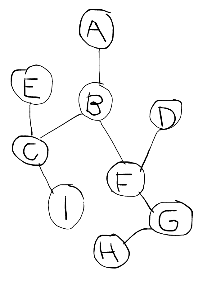 Consider the (cute) network on the right.
- Simulate (on pencil-and-paper) breadth-first search starting from node A when the goal node is H.
- Do the same with depth-first search.
Here's the traversal order in the format node: [node list]:
            BFS            DFS
            a: [b]         a: [b]
            b: [c,f]       b: [f,c]
            c: [f,e,i]     f: [g,d,c]
            f: [e,i,d,g]   g: [h,d,c]
            e: [i,d,g]     h = goal
            i: [d,g]
            d: [g]
            g: [h]
            h = goal
As we discussed above while drinking red wine, search algorithms don't necessarily feel like being very cool AI methods. However, as the next two exercises demonstrate, they can actually be used to solve tasks that -- most of us would admit -- require intelligence.
Let's play. Solve the well-known puzzle Towers of Hanoi. The puzzle involves three pegs, and three discs: one large, one medium-sized, and one small. (Actually, there can be any number of discs but for the pencil-and-paper exercise, three is plenty.)
In the initial state, all three discs are stacked in the first (leftmost) peg. The goal is to move the discs to the third peg. You can only move one disc at a time, and it is not allowed to put a larger disc on top of a smaller disc.
This pretty picture shows the initial state and the goal state:
initial  -     |     |          goal    |     |     -
state:  ---    |     |          state:  |     |    ---
       -----   |     |                  |     |   -----
      =====================         ====================
- Draw a network diagram where the nodes are all the states that can be achieved from the initial state, and the edges represent allowed transitions (moves) between them.
- Simulate breadth-first search in the state space. Note:You don't have to explicitly specify the contents of the queue at each step. It is enough to provide the traversal order.
- Do the same with depth-first search.
- Compare the search methods on two accounts: a) what is the length of the path that each algorithm finds, b) what is the number of states visited during the search. Note: path length and number of visited states are different things.
- Does the result depend on the order in which the neighbors of each node are added into the list?
A bonus exercise: Try to see the symmetry in the state diagram, and generalize to n > 3 discs.
-
Here's the state diagram (from Wikipedia: Towers of Hanoi):
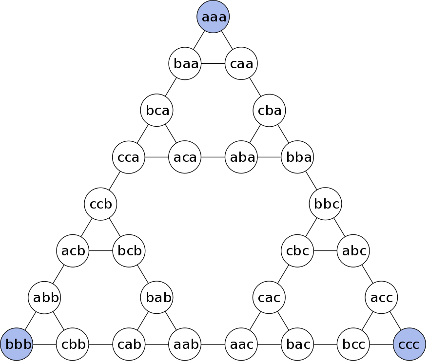
The encoding is such that the first letter in a three-letter sequenceencodes the position of the smallest disk (a= left,b= middle,c= right), the second letter encodes the position of the middle disk, and the third letter encodes the position of the largest disk. Thus, there is a transition from the starting stateaaato statesbaaandcaa, where the smallest disk is move to the middle or the right-most peg respectively. -
BFS visits the states in the following order:
aaa [start], baa, caa, bca, cba, aca, cca, aba, bba,
          ccb, bbc, acb, bcb, abc, cbc, abb, bab, acc, cac,
          bbb, cbb, aab, cab, bcc, ccc [goal]
. Minor differences are possible due to different ordering of the neighbors of each node. -
DFS visits the states in the following order:
aaa [start], caa, cba, bba, bbc, cbc, cac, bac, bcc, ccc
          [goal]
. Here the order in which the neighbors are considered can have a significant effect on the result. In the worst case, all other nodes are visited before expanding the goal node. - a) The path produced by BFS is the one with the least possible transitions, seven. The path produced by DFS, on the other hand, is the same as the sequence of states visited by DFS, which is ten transitions in length. b) BFS visited 25 states altogether while DFS only visited 11 states. So BFS visits much more states but produces a shorter path.
- The number of states visited by BFS varies only slightly, and the path that it produces is always the same (since the shortest path is unique). However, DFS can either go straight to the goal by visiting only the states that are on the shortest path, or it can visit almost all states in the state space, and produce the maximally long path from the start to the goal.
On the bonus exercise, see the Wikipedia page mentioned above.
Alright. So far, we've refreshed BFS and DFS in our memory and applied them to solve some pretty cool applications. To go to the next level, we'll bring out the big guns, and talk about best-first search (which is not abbreviated in order to avoid confusing it with breadth-first search) and the A* algorithm.
Informed Search and A*
Often, different transitions in the state space are associated with different costs. For example, doing a task could take any time between a few seconds and several hours. Or the distance between any two tram stops could be between a hundred meters and half a kilometer. Thus, just counting the number of transitions is not enough.
To be able to take into account different costs, we can apply best-first search, where the node list is ordered by a given criterion. For instance, we can choose to always prefer to expand a path with the minimal incurred total cost counting from the starting node. This is known as Dijkstra's algorithm. In the special case where the cost of all transitions is constant, Dijkstra's algorithm is equivalent to BFS.
The generic search algorithm template above still applies, except for one important detail: In informed search, we'll skip the check that the node hasn't been visited before (so we can drop lines 3, 8, and 9 in the pseudocode above). This guarantees that if a better path to a node that has already been visited is found at a later stage, we make sure to check whether it leads to a better path to the goal.
So except for the above modification, we'll be still using the same search algorithm template. Recall that BFS and DFS were obtained using a queue and a stack as the data structure where the nodes are stored, respectively. In best-first search, the data structure that holds the nodes is a priority queue. When adding nodes to the priority queue on line 14, they are given a cost or a value that is then used to order the nodes in the queue. (Depending on the application and whether the aim is to minimize or maximize the value, the queue can be a min-priority queue or a max-priority queue.)
If you play around with the PathFinding applet for a while, using BFS or Dijkstra's algorithm, you will quickly notice a problem. The search spreads out to all directions symmetrically without any preference towards the goal.
This is understandable since the choice of the next node to expand has nothing to do with the goal. However, if we have some way of measuring, even approximately, which nodes are nearer to the goal, we can use it to guide the search and save a lot of effort by never having to explore unpromising paths. This is the idea behind informed search.
Informed search relies on having access to a heuristic that associates with each node an estimate of the remaining cost from the node to the goal. This can be, for example, the distance between the node and the goal measured as the crow flies (i.e., Euclidean or geodesic distance -- or in plain words, a straight-line distance).
Using the heuristic as the criterion for ordering the nodes in the (min-)priority queue will always expand nodes that appear to be nearer to the goal according to the heuristic. However, this may lead the search astray because the incurred cost of the path is not taken into account. A balanced search that takes both the incurred cost as well as the estimated remaining cost into account is obtained by ordering the (min-)priority queue by
f(node, cost) = cost + h(node),
where cost is the value associated with the node when
it is added to the priority queue, and h(node) is the
heuristic value, i.e., an estimate of the remaining cost
from node to the goal. This is the A* search.
If you try it on
the PathFinding
applet, you will immediately see that it wipes the floor with
other, uninformed search methods.
Games
Next, we will study a classic AI problem: games. The simplest scenario, which we will focus on for the sake of clarity, are two-player, perfect-information games such as tic-tac-toe and chess.
Maxine and Minnie are true game enthusiasts. They just love games. Especially two-person, perfect information games such as tic-tac-toe or chess.
One day they were playing tic-tac-toe. Maxine, or Max as her friends call her, was playing with X. Minnie, or Min as her friends call her, had the Os. The situation was
       O| |O
       -+-+-
       X| |
       -+-+-
       X|O|
Max was looking at the board and contemplating her next move, as it
was her turn, when she suddenly buried her face in her hands in
despair, looking quite like Garry Kasparov playing Deep Blue in
1997.
Yes, Min was close to getting three Os on the top row, but Max could easily put a stop to that plan. So why was Max so pessimistic?
Game Trees
To analyse games and optimal strategies, we will introduce the concept of a game tree. The game tree is similar to a search tree. (Remember that you should also study the lecture slides in addition to this material. Some material may be discussed in one but not the other.) The different states of the game are represented by nodes in the game tree. The "children" of each node N are the possible states that can be achieved from the state corresponding to N. In board games, the state of the game is defined by the board position and whose turn it is.
Consider, for example, the following game tree which begins
not at the root but in the middle of the game (because otherwise,
the tree would be way too big to display).
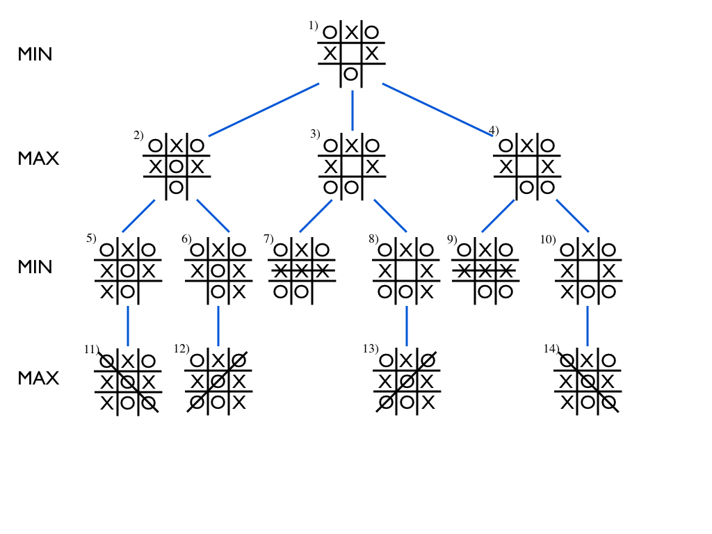
The game continues at the board position shown in the root node,
numbered as (1) at the top, with Min's turn to place O at any of the
three vacant cells. Nodes (2)--(4) show the board positions
resulting from each of the three choices respectively. In the next
step, each node has two possible choices for Max to play X each,
and so the tree branches again.
The game ends when either player gets a row of three, or when there are no more vacant cells. When starting from the above starting position, the game always ends in a row of three.
Now consider nodes (5)--(10) on the second layer from the bottom. In nodes (7) and (9), the game is over, and Max wins with three X's in a row. In the remaining nodes, (5), (6), (8), and (10), the game is also practically over, since Min only needs to place her O in the only remaining cell to win. We can thus decide that the end result, or the value of the game in each of the nodes on the second level from the bottom is determined. For the nodes that end in Max's victory, we'll say that the value equals +1, and for the nodes that end in Min's victory, we'll say that the value is -1.
More interestingly, let's now consider the next level of nodes towards the root, nodes (2)--(4). Since we decided that both of the children of (2), i.e., nodes (5) and (6), lead to Min's victory, we can without hesitation attach the value -1 to node (2) as well. For node (3), the left child (7) leads to Max's victory, +1, but the right child (8) leads to Min winning, -1. However, it is Max's turn to play, and she will of course choose the left child without hesitation. Thus, every time we reach the state in node (3), Max wins. Thus we can attach the value +1 to node (3).
The same holds for node (4): again, since Max can choose where to put her X, she can always ensure victory, and we attach the value +1 to node (4).
So far, we have decided that the value of node (2) is -1, which means that if we end up in such a board position, Min can ensure winning, and that the reverse holds for nodes (3) and (4): their value is +1, which means that Max can be sure to win if she only plays her own turn wisely.
Finally, we can deduce that since Min is an experienced player, she can reach the same conclusion, and thus she only has one real option: give Max an impish grin and play the O in the middle of the board.
In the diagram below, we have included the value of each node as
well as the optimal game play starting at Min's turn in the root
node.
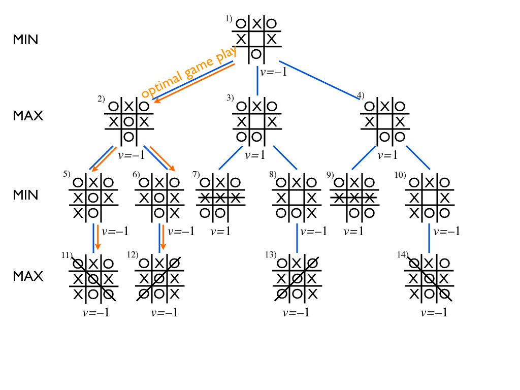
The value of the root node, which is said to be the value of the game, tells us who wins (and how much, if the outcome is not just plain win or lose): Max wins if the value of the game is +1, Min if the value is -1, and if the value is 0, then the game will end in a draw. This all is based on the assumption that both players choose what is best for them.
The optimal play can also be deduced from the values of the nodes: at any Min node, i.e., node where it is Min's turn, the optimal choices are given by those children whose value is minimal, and conversely, at any Max node, where it is Max's turn, the optimal choices are given the the children whose value is maximal.
Minimax Algorithm
We can exploit the above concept of the value of the game to obtain an algorithm with optimal game play in, theoretically speaking, any deterministic, two-person, perfect-information game. Given a state of the game, the algorithm simply computes the values of the children of the given state and chooses the one that has the maximum value if it is Max's turn, and the one that has the minimum value if it is Min's turn.
The algorithm can be implemented using the neat recursive functions below for Max and Min nodes respectively. This is known as the Minimax algorithm (see Wikipedia: Minimax).
    max_value(node):
1:     if end_state(node): return value(node)
2:     v = -Inf
3:     for each child in node.children():
4:        v = max(v, min_value(child))
5:     return v
    min_value(node):
1:     if end_state(node): return value(node)
2:     v = +Inf
3:     for each child in node.children():
4:        v = min(v, max_value(child))
5:     return v
Let's return to the tic-tac-toe game described in the beginning of this section. To narrow down the space of possible end-games to consider, we can observe that Max must clearly place an X on the top row to avoid imminent defeat:
       O|X|O
       -+-+-
       X| |
       -+-+-
       X|O|
Now it's Min's turn to play an O. Evaluate the value of this state
of the game as well as the other states in the game tree where the
above position is the root, using the Minimax algorithm.
Here's the game tree with the values of each node.
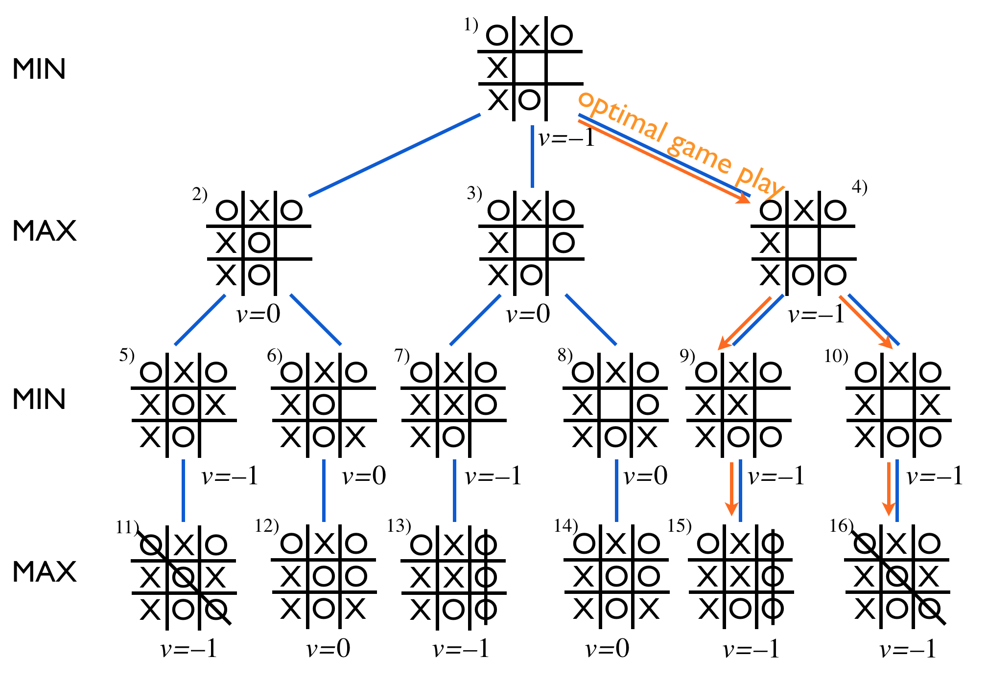
As you can see, Max has all the reason to be serious since by playing in the bottom-right corner (Node (4)), Min can guarantee a win (just follow the orange arrows). The inevitable victory of Min can also be seen from the value of the game at the root node which is –1.
As stated above, the Minimax algorithm can be used to implement optimal game play in any deterministic, two-player, perfect-information game. Such games include tic-tac-toe, connect four, chess, Go, etc. (Rock-paper-scissors is not in this class of games since it involves information hidden from the other player; nor are Monopoly or backgammon which are not deterministic.) So as far as this topic is concerned, is that all folks, can we go home now?
The answer is that in theory, yes, but in practice, no. In many games, the game tree is simply way too big to traverse in full. For example, in chess the average branching factor, i.e., the average number of children (available moves) per node is about 35. That means that to explore all the possible scenarios up to only two moves ahead, we need to visit approximately 35 x 35 = 1225 nodes -- probably not your favorite pencil-and-paper homework exercise... A look-ahead of three moves requires visiting 42875 nodes; four moves 1500625; and ten moves 2758547353515625 (that's about 2.7 quadrillion) nodes.
In Go, the average branching factor is estimated to be about 250. Go means no-go for Minimax.
Next, we will learn a few more tricks that help us manage massive game trees, and that were crucial elements in IBM's Deep Blue computer defeating the chess world champion, Garry Kasparov, in 1997.
Depth-limited minimax and heuristic evalution criteria
If we can afford to explore only a small part of the game tree, we need a way to stop the minimax recursion before reaching an end-node, i.e., a node where the game is over and the winner is known. This is achieved by using a heuristic evaluation function that takes as input a board position, including the information about which player's turn is next, and returns a score that should be an estimate of the likely outcome of the game continuing from the given board position.
Good heuristics for chess, for example, typically count the amount of material (pieces) weighted by their type: the queen is usually considered worth about two times as much as a rook, three times a knight or a bishop, and nine times as much as a pawn. The king is of course worth more than all other things combined since losing it amounts to losing the game. Further, occupying the strategically important positions, e.g., near the middle of the board, is considered an advantage.
The minimax algorithm presented above requires minimal changes to obtain a depth-limited version where the heuristic is returned at all nodes at a given depth limit.
Alpha-beta pruning
Another breakthrough in game AI, proposed independently by several researchers including John McCarthy in and around 1960, is alpha-beta pruning. For small game trees, it can be used independently of the heuristic evaluation method, and for large trees, the two can be combined into a powerful method that has dominated the area of game AI for decades.
A good example of the idea behind alpha-beta-pruning can be seen in the tic-tac-toe game tree that we discussed above -- scroll up and let the image of the root node burn into your retina.
Now simulate the Minimax algorithm at the stage where the value of
the left child node, -1, has been computed and returned to the
min_value function. The next step would be to
call max_value to compute the value of the middle
child. But hold on! If the left child guarantees victory for Minnie,
what does it matter how the game ends if she chooses to play any
other way? As soon as the algorithm finds a child node with the best
possible outcome for the player whose turn it is, it can make a
choice and avoid computing the values of all the other child nodes.
To implement this in a similar fashion as the Minimax algorithm
requires small changes in the min_value and
max_value functions. Understanding the connection
between these changes and the principle illustrated by the above
pruning example is not as easy as it may sound, so please pay
close attention to this topic and work out the examples and
exercises with care.
    max_value(node, alpha, beta):
1:     if end_state(node): return value(node)
2:     v = -Inf
3:     for each child in node.children():
4:        v = max(v, min_value(child, alpha, beta))
5:        alpha = max(alpha, v)
6:        if alpha >= beta: return v
7:     return v
    min_value(node, alpha, beta):
1:     if end_state(node): return value(node)
2:     v = +Inf
3:     for each child in node.children():
4:        v = min(v, max_value(child, alpha, beta))
5:        beta = min(beta, v)
6:        if alpha >= beta: return v
7:     return v
An important thing to remember is that the alpha value
is updated only at the Max nodes, and the beta value is
updated only at the Min nodes. The updated values are passed as
arguments down to the children, but not up to the calling parent
node. (That is, the arguments are passed as values, not as
references in programming lingo.)
The interpretation alpha and beta is that
they provide the interval of possible values of the game at the node
that is being processed:
alpha ≤ value ≤ beta. This interval
is updated during the algorithm, and if at some point, the interval
shrinks so that alpha = beta, we know the value and
can return it to the parent node without processing any more
child nodes. It can also happen that alpha > beta,
which implies that the current node will never be visited in
optimal game play, and its processing can likewise be aborted.
When starting the recursion at the root node, we use the minimum and
maximum value of the game as the alpha
and beta values respectively. For tic-tac-toe and
chess, for instance, where the outcome is plain win/loss, this
is alpha = -1 and beta = 1. If the range
of possible values is not specified in advance, we initialize
as alpha = -∞ and beta = ∞.
It is useful to work out a few examples to really understand the
beauty of alpha-beta pruning. Here's another tic-tac-toe
example.
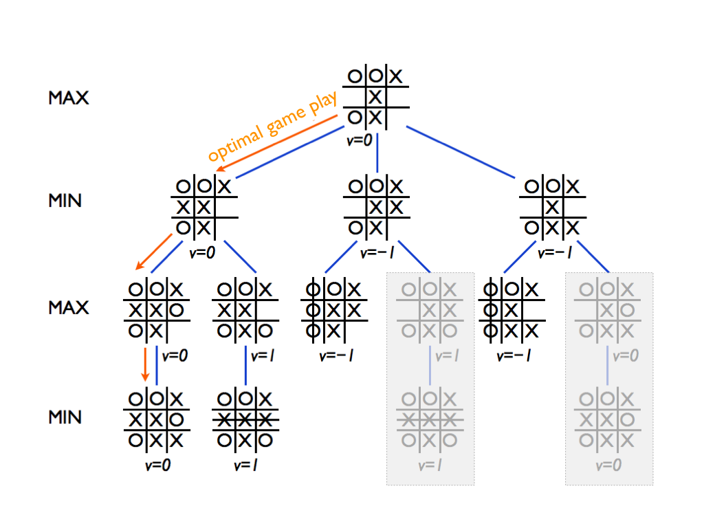
You should simulate the algorithm to see that the two branches that are grayed out indeed get pruned -- therefore, it is actually a bit misleading to even show their minimax values since the algorithm never computes them.
Remember that the Max nodes (such as the root node) only update
the alpha value and pass it down to the next
child node. Check that you reach a situation where
alpha=0 and beta=-1 in a
Min node. Actually you should reach such a situation twice.
Maxine wants to try again -- best out of three! Minnie agrees and after a while, they arrive at the following position
       O|X|O
       -+-+-
       X| |X
       -+-+-
        |O|
It's again Min's turn to play an O. Evaluate the value of this state
of the game as well as the other states in the game tree where the
above position is the root, using alpha-beta pruning. Start the
recursion by calling min-value(root, -1, 1) where
root is the above board position.
What is the value of the game, and what are the optimal moves?
As was stated in the exercise, the recursion
is started by calling
min-value for the root node (Node (1) below) with
arguments
alpha=-1, beta=1. These values are then passed to the
child nodes, starting with the leftmost child (Node (2)), and from
it further down all the way to the leaf node (5). The return value,
which is passed up the parent node (3), is –1 since in this
case, Min wins with three Os in a row. Strictly speaking, this
already causes pruning to occur in Node (3): it is a Min node, and
thus it updates its beta value, and the beta value becomes
–1. The test alpha =-1 ≤ beta=-1 (line 6
in the pseudocode) triggers the return condition. However, the
effect is null since there wouldn't have been any other children of
Node (3) anyway.
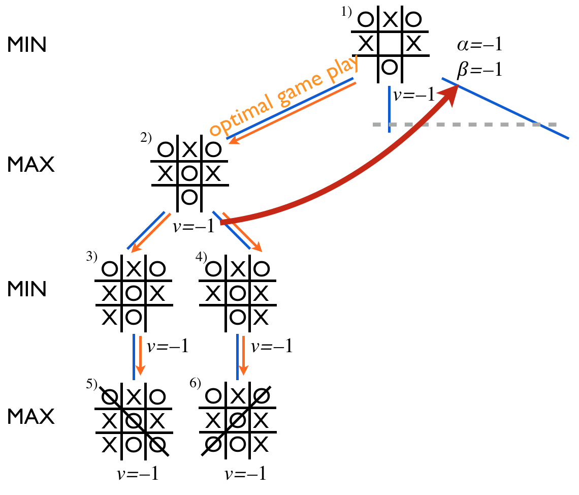
Next, Node (3) returns the value –1 to its parent, Node (2). As a Max node, Node (2) would update its alpha value but since the value returned by the child is –1 which is already the same as the current alpha value, no update occurs (line 5 in the pseudocode). The processing of nodes (4) and (6) is analogous to that of nodes (3) and (5) respectively.
Interesting things start to happen in the root node when the value
–1 is returned from Node (2). The root node is a Min node and
it updates its beta value to be beta=-1 (line 5 in the
pseudocode), and therefore, the test alpha=-1 ≤
beta=-1 again triggers pruning and the other branches of the
tree need not be traversed at all!
The optimal game play can now be obtained by always choosing the child node with the minimum (maximum) value in Min (Max) nodes among the child nodes that were visited. The result is guaranteed to be the same as that of the Minimax algorithm, i.e., optimal play for both players. For Max this is bad news: it's Min's victory even best-out-of-three...
Notice that while the left-to-right order of the children of each node, i.e., the order in which the children are processed in the loop on lines 4--6, is arbitrary, it can have significant impact on which branches are pruned.
Now we feel confident enough about concepts and ideas behind the Minimax algorithm and alpha-beta pruning that we can start programming. We'll implement a tic-tac-toe bot.
Download the starter package
AlphaBeta.zip,
unzip it, and open the AlphaBeta folder in VS Code
(or another editor). The package contains starter code under
src/ and local tests under test/.
- First implement the basic framework for the game: a data structure (class) for board positions, the functions for checking whether either player has a row of three, and a function for producing the list of children for a given board position.
- Then implement the Minimax algorithm according to the pseudo-code given above. The algorithm should return for any given board position, the value of the game: -1, 0, or 1.
- Using the previous step, modify the program so that it also outputs the optimal move for the player whose turn it is (which is given as an input, of course). You can do this by keeping record of the child node that yields the highest (lowest) value in a Max (Min) node.
- You can test the solution at this stage by using it to solve the above pencil-and-paper exercises.
- As the culmination of this exercise, modify the algorithm to
implement alpha-beta pruning as detailed in the pseudo-code
above. To see whether you gain any speed-up, you can see how
long the algorithm runs (or how many recursive function calls
are performed) with or without alpha-beta pruning -- simply
comment out line 6 with the test
alpha >= betato revert back to vanilla Minimax.
AlphaBeta folder, run the local tests with:
python3 -m testrunnerExample solutions for Python.
This is a bonus exercise. The Games section above focuses on zero-sum games such as tic-tac-toe. Many real interactions are different: both players can gain by cooperating, or both can lose by cheating.
Play Nicky Case's interactive guide The Evolution of Trust (about 30 minutes). It is a short demo of the iterated Prisoner's Dilemma and how trust and cooperation can evolve — or collapse. Just play through it and enjoy the demo; there is nothing to hand in.
This is the end of Week 1. You should now be familiar with what AI is, how to solve problems by search (including A*), and how to play games with minimax and alpha-beta pruning.