Modern Architectures and Foundation-Model Applications

Episode 9: Attention and self-attention

Part 4 introduced embeddings as learned vector representations. A static embedding cannot adapt its meaning to the surrounding sequence. Attention solves this problem by letting each position select and combine information from other positions. Episode 9 develops this mechanism and shows why it became the foundation of the Transformer.

One word, different context

Consider the word bank in “the bank approved the loan” and “we sat on the river bank.” A static lookup gives the same initial vector in both sentences. Attention creates a contextual representation by combining information from the surrounding tokens with different strengths.

Why Do We Need Attention?

First, let's recall that before 2017 (when the original paper introducing the transformer architecture was published), the primary approach for handling sequences was using recurrent neural networks (RNNs). However, this approach has several well-known limitations:

• Memory bottleneck: RNNs store all information about the sequence in a hidden state, which is updated at each step. If the model needs to "remember" something that happened hundreds of steps earlier, this information must be retained in the hidden state without being replaced by new data. This means either having an extremely large hidden state or accepting inevitable information loss.
• Sequential processing: Training recurrent networks is difficult to parallelize. To compute the hidden state of the RNN layer at step i+1, you must first compute the state for step i. Thus, processing a batch of sequences with a length of 1000 requires 1000 sequential operations, making training time-consuming and inefficient on GPUs, which are optimized for parallel computations.

These issues make it challenging to apply RNNs to truly long sequences: even if you wait for training to finish, your model, by design, will inevitably lose information from the beginning of the text. Ideally, we want a way to "read" a sequence such that at any moment, the model can refer to any previous point in constant time, without losing information.

This is exactly what the self-attention mechanism at the core of transformers enables. As we will see later, this mechanism is effective for natural language processing. The same idea later transferred to many other domains.

Below is the architecture of the transformer model, as presented in the original paper:

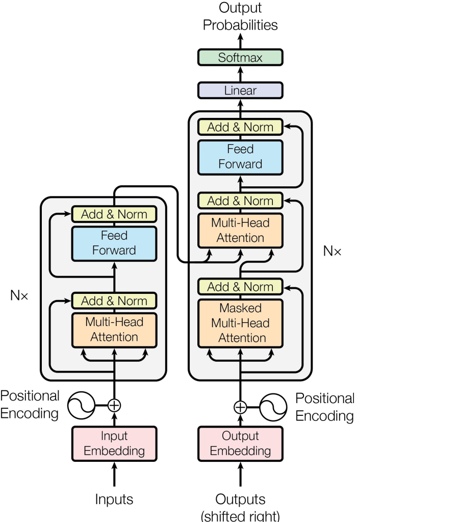
Transformer Encoder and Decoder

On the left side of the diagram, we see the structure of the encoder. It sequentially applies N blocks to the input sequence:

Each block outputs a sequence of the same length. It contains two key layers: multi-head attention and feed-forward. After each of these layers, the input is added back to the output (this standard approach is called a residual connection), and then the activations pass through a layer normalization layer. This part is labeled as "Add & Norm" in the diagram.

The decoder follows a similar structure, but each of its N blocks contains two multi-head attention layers, one of which incorporates the encoder's outputs.

Now, let's take a closer look at each of the key components of this mechanism.

Attention Layer

The first part of the Transformer block is the self-attention layer. Unlike standard attention mechanisms, its output consists of new representations for elements from the same input sequence, where each element directly interacts with every other element.

More specifically, the computation of attention for a sequence involves three trainable matrices: W_Q, W_K, W_V. Each input element representation xi is multiplied by these matrices, producing row vectors qi, ki, vi (where i is the index of the element). These vectors are referred to as query, key, and value, respectively.

Their roles can be loosely described as follows:

• q_i — the query to a database.
• k_i — the keys of stored values in the database, used for lookup.
• v_i — the actual stored values.

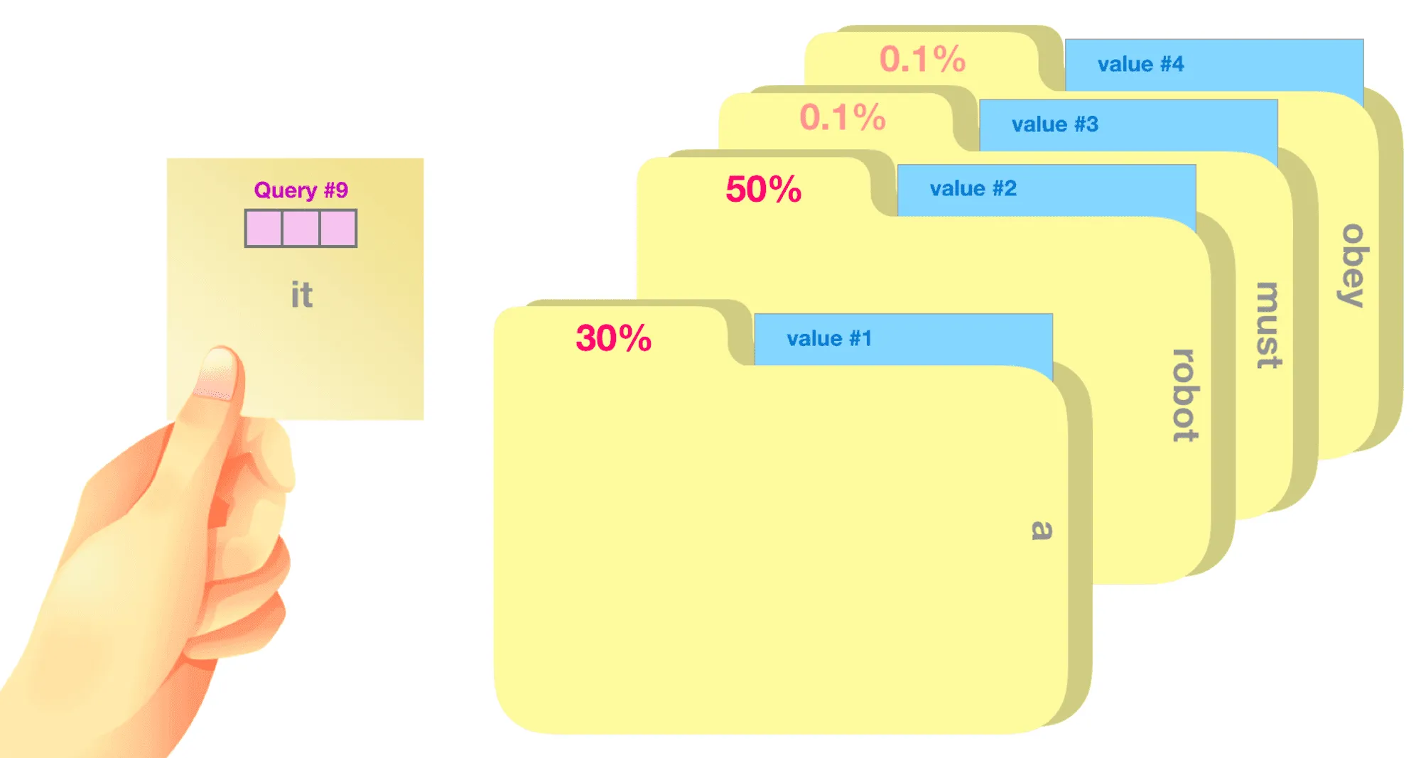
The closeness of a query to a key can be determined using a dot product:

self-attention weights_i = softmax(C ⟨q_i, k₁⟩, C ⟨q_i, k₂⟩, …),

where C is a normalization constant. In the original paper, the normalization constant was chosen as the square root of the key and value dimension √d_k.

Now, we sum the values v_i with the obtained coefficients. This is the output of the self-attention layer. In matrix form, it can be written as:

self-attention(Q, K, V) = softmax (QK^T / √d_k) V,

where Q, K, V are matrices of queries, keys, and values, respectively, with q_i, k_i, v_i stored as row vectors, and softmax is applied row-wise.

Attention Layer in the Decoder

As mentioned earlier, one of the attention layers in the decoder is a cross-attention layer, where the queries are taken from the output sequence, while the keys and values come from the input (i.e., from the encoder's outputs).

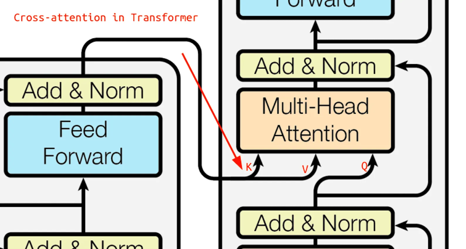
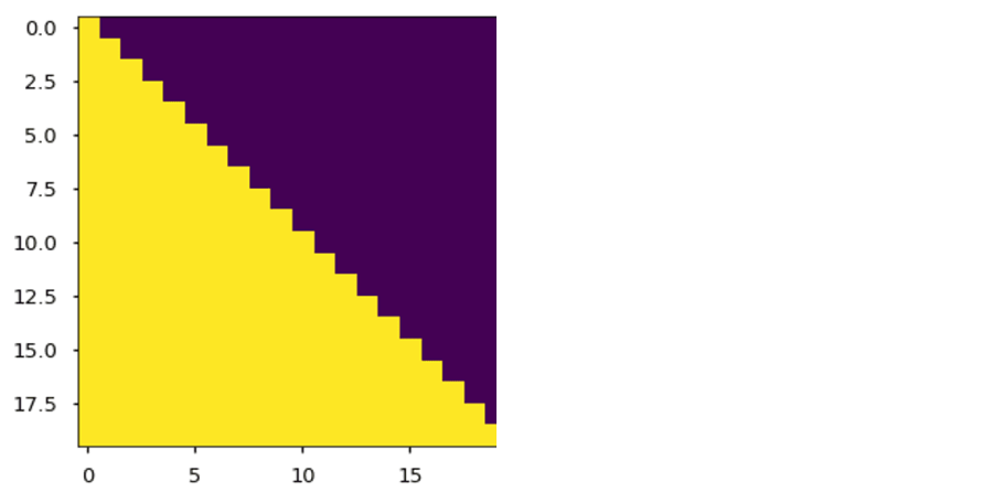
Another key feature of the decoder's attention is that, in the form described above, each token would have access to the entire sequence, which is undesirable for the decoder. Indeed, during generation, we produce tokens one step at a time, and having access to future tokens during training would lead to information leakage and poor model performance.

To prevent this issue, an autoregressive mask is applied to attention during training, manually setting weights for future tokens to -∞ before the softmax operation, ensuring their probabilities become zero after softmax. As shown in the image below, this mask has a lower triangular shape.

Multi-Head Attention

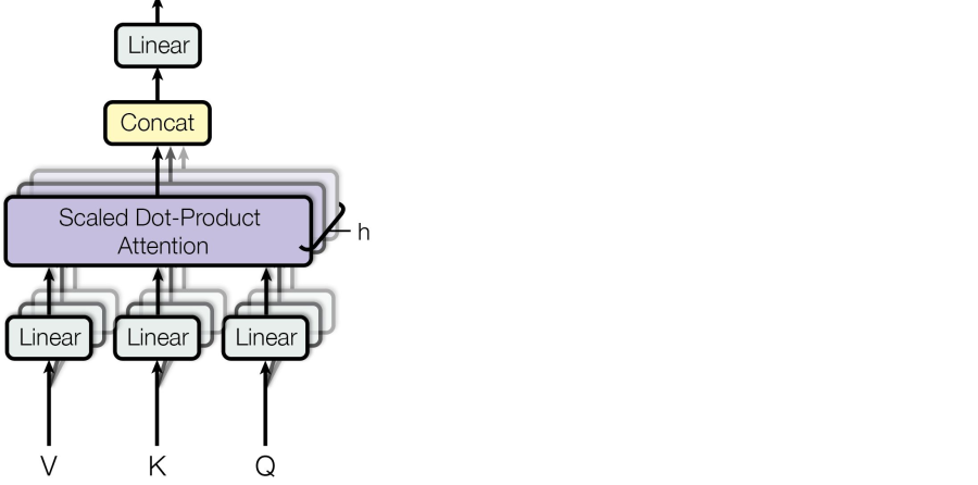
A single set of matrices Q, K, and V can capture only one type of dependencies between tokens, and these matrices extract only a limited range of information from the input representations. To address this limitation, the authors of the Transformer architecture introduced the concept of multi-head attention.

Instead of using a single attention mechanism, multiple parallel attention layers (or "heads") with different learned weights are applied simultaneously. The results from all heads are then concatenated and passed through a linear transformation. This allows the model to attend to different parts of the input sequence and capture multiple relationships in parallel.

Efficiency

The approach of processing entire sequences using attention eliminates the concept of a hidden state that updates recurrently. Instead, each token can directly "read" any part of the sequence that is most useful for prediction. In particular, the absence of recurrence allows us to apply the layer to the entire sequence simultaneously, leveraging matrix multiplications that parallelize efficiently.

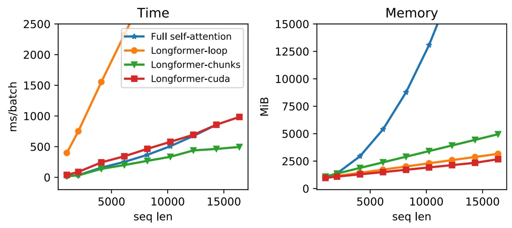
However, we must consider memory and time complexity costs: since each element in the sequence interacts with every other element, it is easy to show that the computational complexity of self-attention is O(n^2) with respect to sequence length. Additionally, naive implementations that construct a full attention matrix also require O(n^2) memory.

Optimizing the computational efficiency of attention has led to numerous research efforts, both engineering-focused and architectural. Some approaches reduce self-attention runtime to linear complexity or significantly improve memory efficiency by leveraging GPU memory hierarchy.

For example, the graphs below compare the runtime and memory consumption of a standard transformer with the mechanism introduced in Longformer:

Episode 10: Transformers, BERT and GPT

Attention is one component of a Transformer block. Episode 10 examines how attention, feed-forward layers, residual connections and normalization form complete encoder and decoder architectures. It then compares BERT-style representation learning with GPT-style autoregressive generation and considers applications beyond text.

From tokens to contextual predictions

The same general pipeline supports different objectives. An encoder can produce contextual representations for classification or retrieval. An autoregressive decoder uses a causal mask and predicts the next token repeatedly. Encoder-decoder models transform one sequence into another, as in translation. The details below explain the operations repeated inside each block.

Inside the Transformer block

The second component of the transformer block is the feed-forward network (FFN), which consists of two fully connected layers applied independently to each element of the input sequence. In modern architectures, the size of the intermediate representation (i.e., the output of the first layer) is often significantly larger—typically four times the output size of the block.

Because of this, the computational cost of FFN should not be underestimated: despite the quadratic complexity of self-attention, in large models or for short sequences, the FFN can take significantly more time than self-attention. Mathematically, the FFN is represented as:

FFN(x) = act(xW_1 + b_1)W_2 + b_2

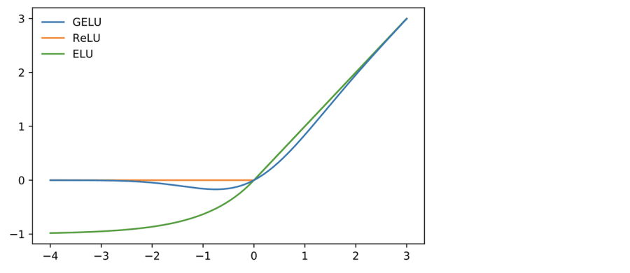
The activation function act in the FFN has varied over time. Initially, ReLU was widely used, but the community later adopted GELU (Gaussian Error Linear Unit), which follows the formula:

GELU(x) = x \cdot \Phi(x)

where \Phi is the cumulative distribution function of the standard normal distribution.

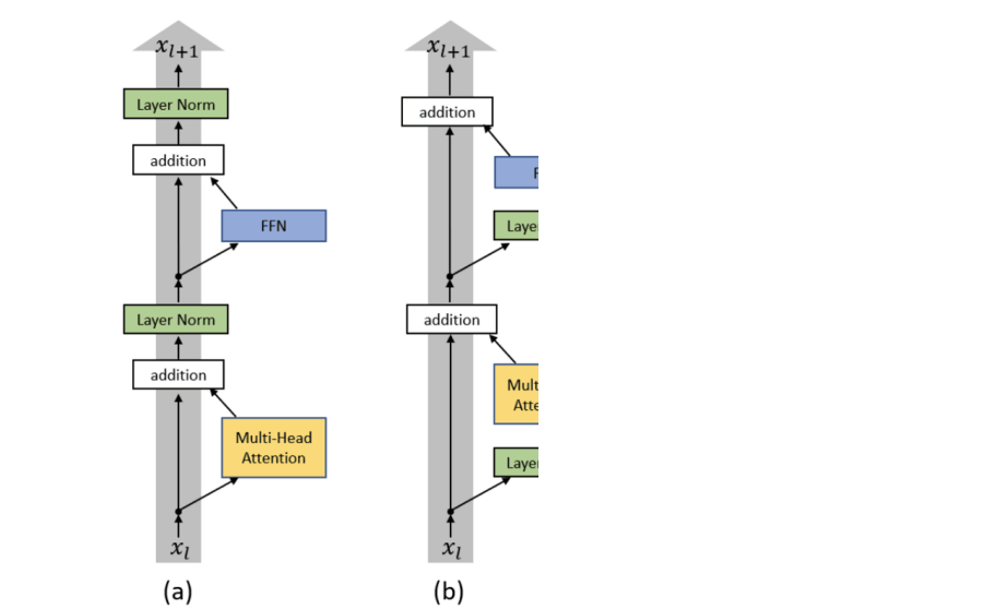
Let's say a few words about layer normalization: as demonstrated in several research papers, its placement within the residual connection is crucial. The standard transformer architecture employs the PostLN formulation, where normalization is applied after the residual connection.

However, this approach can be quite unstable when training deep models with a large number of layers. Instead, an alternative approach, PreLN (shown on the right in the image below), applies normalization to the input of the residual connection.

BERT and GPT

Transformer-based models wouldn’t be as interesting if almost all modern NLP tasks weren’t being solved using this architecture. The rapid rise in popularity of self-attention was driven by two well-known model families: BERT and GPT. These can be seen as the encoder and decoder of the Transformer, which later evolved into independent architectures.

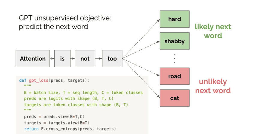
Chronologically, GPT (Generative Pretrained Transformer) was introduced first. It is a standard language model implemented as a stack of Transformer decoder layers.

The training objective is simply next-token prediction, meaning it performs multi-class classification over a vocabulary at each step. A key feature of GPT is the use of a lower-triangular attention mask: without it, future tokens would be visible to past ones, causing a data leakage issue.

The trained model can be used for text generation and tasks that rely on it. Even ChatGPT, which is fine-tuned with special instruction-based training, differs only slightly from the base GPT model.

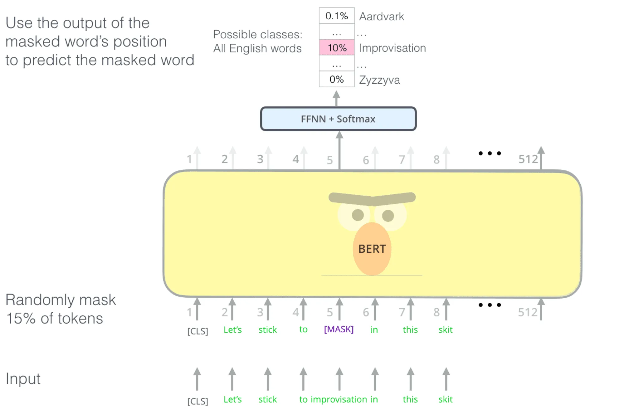
As the name suggests, the Bidirectional Encoder Representations from Transformers (BERT) model differs from GPT in its bidirectional attention: this means that while processing the input sequence, all tokens can leverage information from each other.

This makes BERT particularly suitable for tasks where predictions need to be made based on the entire input without text generation. Examples include sentence classification and document similarity search. However, BERT does not generate text from scratch.

Instead, BERT is trained with two key objectives:

• Masked Language Modeling (MLM): Predicting randomly masked words based on their surrounding context (illustrated in the image below).
• Next Sentence Prediction (NSP): Determining whether two text fragments logically follow each other.

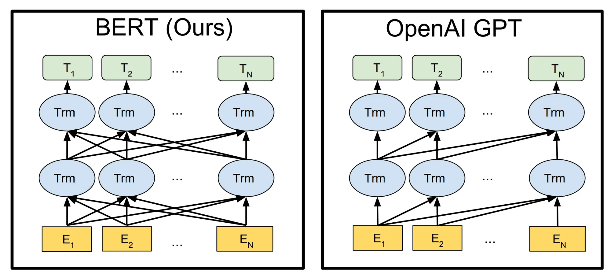
The key difference between BERT and GPT models is not just in their training objectives or applications but primarily in the type of attention mechanisms they use. This distinction is illustrated in the image below.

Training Nuances

Unfortunately, if you simply implement a Transformer neural network and attempt to train it using conventional hyperparameters from other architectures, you are highly likely to encounter failure. The optimization process for such models often requires adjustments, and neglecting these details can result in significant quality degradation or even unstable training.

One critical factor is the batch size. Almost all modern Transformer models are trained on extremely large batches, sometimes reaching millions of tokens in the largest language models. Since no modern GPU can handle such large batches in a single step, techniques like gradient accumulation are commonly used to accumulate gradients over micro-batches before performing an update.

Recent research also suggests increasing the batch size dynamically during training. The idea is that during early training stages, making more frequent gradient descent steps is crucial, while in later stages, it is more important to have an accurate gradient estimation.

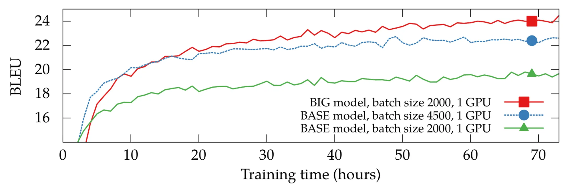
Another crucial factor is the choice of optimizer and learning rate schedule. Training a Transformer with standard SGD is highly unlikely to succeed. In the original Transformer paper, the Adam optimizer was used, and to this day, it remains the standard choice.

However, for large batch sizes, Adam sometimes struggles, leading researchers to use alternatives such as LAMB, which normalizes weight updates for each layer to stabilize training.

Transformers Beyond Text

Naturally, the remarkable success of this family of architectures in various text-related tasks did not go unnoticed by researchers in other domains. One of the most prominent areas where Transformer-based models have found new applications is undoubtedly computer vision.

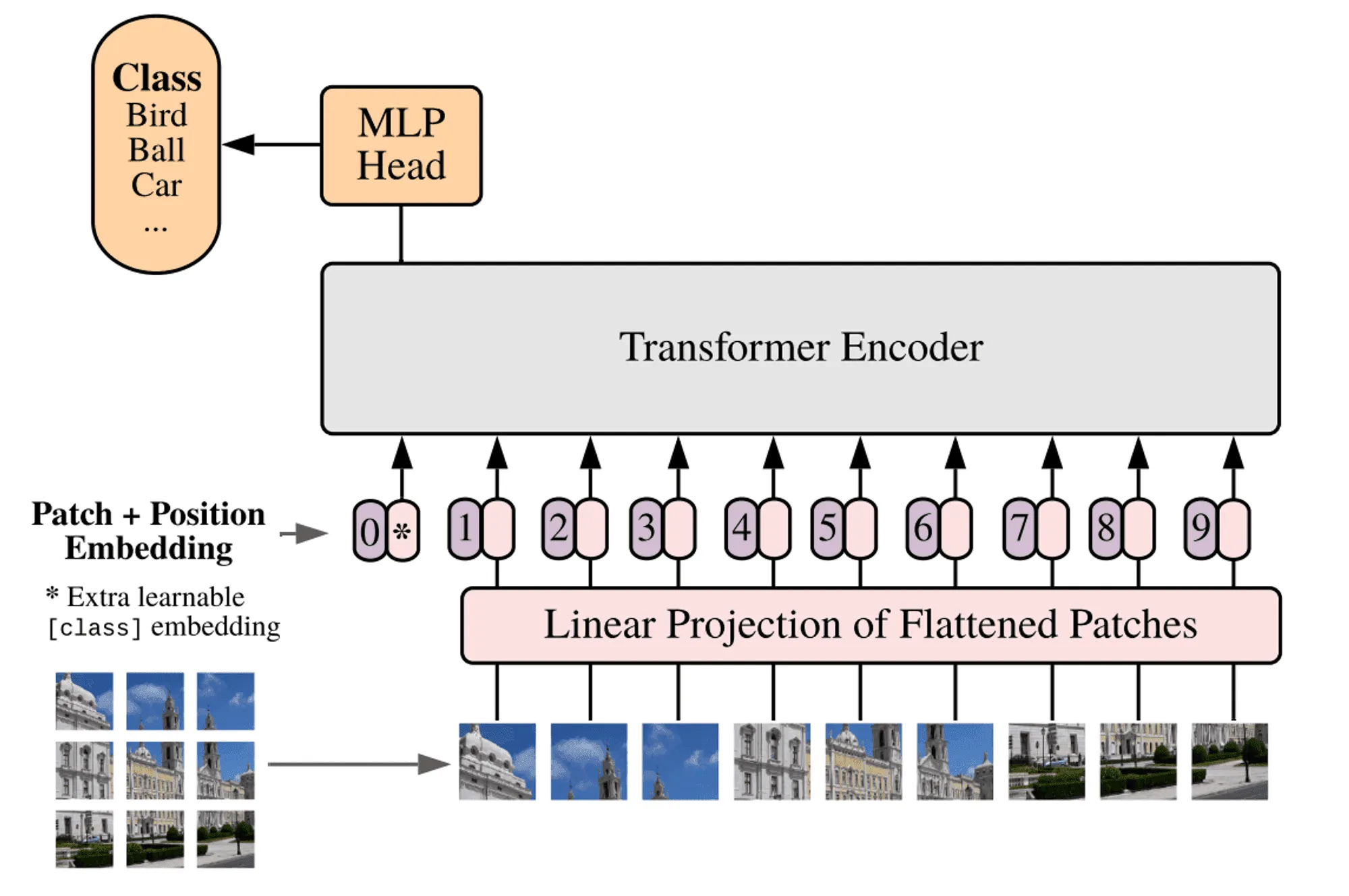
For example, the ViT (Vision Transformer) architecture once broke classification accuracy records on image datasets by leveraging the self-attention mechanism for images divided into multiple patches—square-shaped segments.

As the authors of the paper explain, the idea of using Transformer architecture in vision emerged after observing the success of such models in NLP. The use of a general approach like self-attention allows architectures to bypass the need for explicitly encoding task-specific properties (also known as inductive bias), provided there is sufficient training time, a large number of parameters, and an extensive dataset.

Transformers in Image Generation and Reinforcement Learning

Transformers also serve as the foundation for the generative component of DALL-E— a model that sparked a wave of research in text-to-image generation in recent years. Conceptually, DALL-E is quite simple: it can be viewed as an autoregressive "language model" that generates an image one "visual token" at a time.

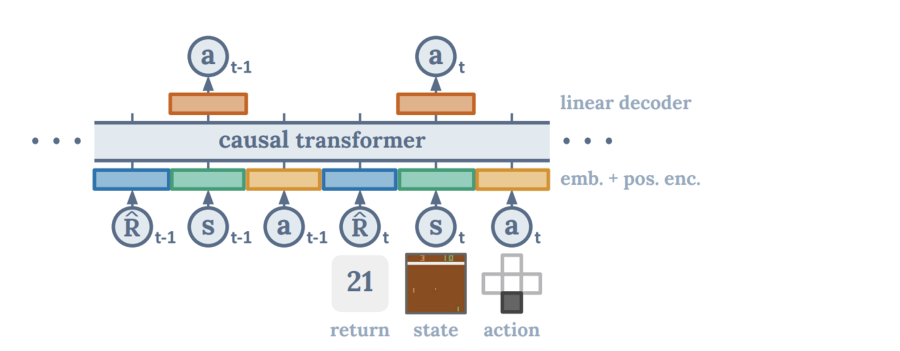
Transformers are also applied in reinforcement learning. A notable example is the Decision Transformer paper, which proposes using autoregressive modeling with this architecture to construct an agent.

The authors demonstrated that the same approach used for text generation can be applied to predicting actions in a dynamic environment. As shown in the image below, the model sequentially receives standard triplets of encoded states, current actions, and rewards, and at each step, it outputs the next action.

Running Language Models Locally

The exercises below let you run language models on your own computer. Running a small or quantized model does not require an expensive GPU. Training a modern large language model from scratch is a very different task: it requires enormous datasets, memory, and costly clusters of GPUs. We will therefore use small models to explore the same basic ideas on an accessible scale.

NanoGPT: a small and transparent GPT implementation

Andrej Karpathy's nanoGPT is deprecated and no longer maintained. The repository is still useful because it is small enough to inspect. The core ideas are still the ones used in modern GPT systems: Transformer blocks, causal self-attention, next-token prediction, sampling, and fine-tuning.

To make these exercises reproducible, use the fixed commit shown below instead of the changing default branch. We use the smallest GPT-2 checkpoint and short runs so a laptop CPU is enough.

Episode 11: Foundation models and generative applications

From task-specific models to foundation models

A task-specific model is trained for one defined input-output problem. A foundation model is pretrained on broad data at sufficient scale to support many downstream tasks. The term was developed systematically in the Stanford report on foundation models. The same base model can be adapted for classification, retrieval, generation, question answering or interaction. This reuse changes the unit of AI development: practitioners increasingly select, prompt, adapt and evaluate pretrained models rather than train every system from scratch.

Scale alone does not define a foundation model. The central feature is broad transfer. Pretraining learns representations and behavioural regularities from a general objective, such as predicting missing or next tokens. Downstream use then specifies the task through prompts, demonstrations, retrieved context or additional training.

Transfer and adaptation

Method	What changes	Main trade-off
Prompting	The input instructions and examples	Fast, but sensitive to wording and model capability
Retrieval-augmented generation	External evidence is added to the context	More current and grounded, but retrieval can fail
Fine-tuning	Some or all model parameters	Stronger specialization, but requires data and evaluation
Parameter-efficient tuning	A small set of added or selected parameters	Cheaper adaptation with less freedom than full fine-tuning

Transfer works when knowledge acquired during pretraining is relevant to the new task. It can fail under domain shift, unfamiliar languages or modalities, and tasks requiring knowledge absent from the training data. Adaptation must therefore be evaluated on the actual population and setting in which the system will operate.

Multimodal foundation models

Multimodal models connect representations from text, images, audio, video, actions or sensor data. Some map different modalities into a shared embedding space, making cross-modal retrieval possible. Others accept several modalities as context and generate text, images, audio or actions. A vision-language model, for example, may answer questions about an image because visual features have been aligned with language representations.

Multimodality does not guarantee a unified understanding of the world. Models may rely on shortcuts, miss spatial or temporal relations, or produce fluent descriptions unsupported by the input. Evaluation should test grounding, robustness and performance across modalities rather than assess language quality alone.

Generative models

Up until now, you have studied machine learning models that primarily predict certain characteristics of objects, such as class labels or regression targets. These types of tasks are referred to as discriminative modeling.

However, there are also inverse problems where an object needs to be created based on certain characteristics or the probability distribution of objects needs to be estimated. This is known as generative modeling—the key aspects of which we will explore in this section.

Training generative models is significantly more challenging than training discriminative models. The latter operate with much simpler distributions. For instance, predicting the probability of a specific digit appearing in an image is much easier than generating an image with the desired digit. Despite these challenges, generative models have achieved remarkable success in recent years, enabling the creation of images that are nearly indistinguishable from real photographs.

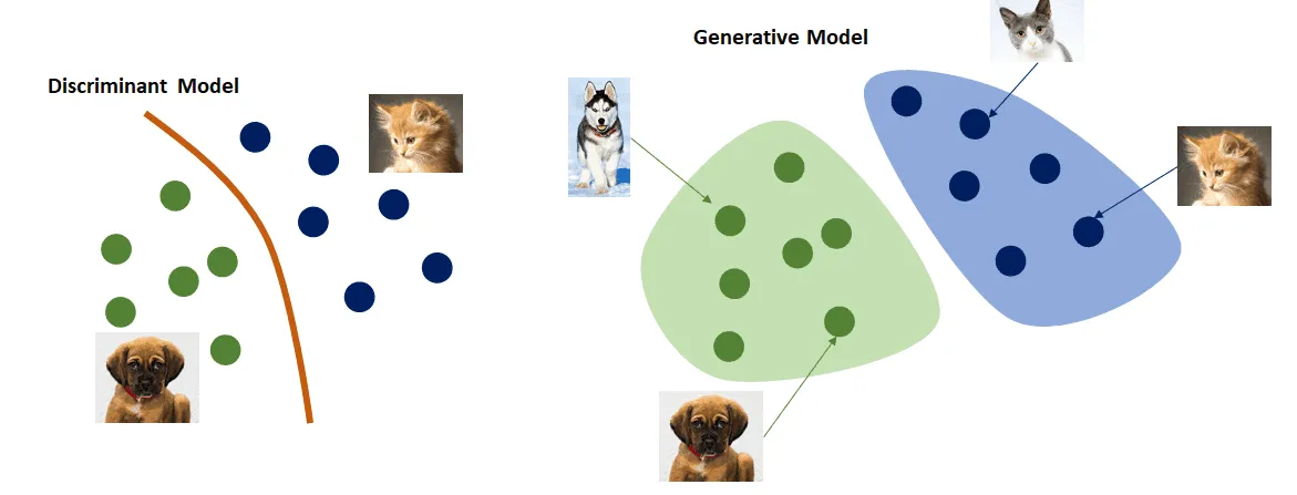
Generative models help solve a variety of tasks, which we will explore further. The most fundamental task is approximating the data distribution and generating new data.

Suppose we have a dataset of handwritten digit images. We assume that this dataset is sampled from a larger population (i.e., the entire set of possible images). Our goal is to model the distribution of this population in some way.

We can achieve this using two approaches:

• Explicit modeling: In this case, we construct and estimate the probability density function p(x). From this distribution, we can sample new objects. Examples of such models include:
  • Autoregressive models (e.g., PixelCNN++, Video Transformer)
  • Diffusion models
  • Models based on normalizing flows
  • Variational autoencoders
• Implicit modeling: In this approach, we do not directly estimate the probability density function, but we can still sample new objects from the learned distribution. In our example of handwritten digits, we would be able to generate similar images. A notable example of such models is Generative Adversarial Networks (GANs).

Discriminative vs. Generative Models

Let's formalize the difference between discriminative and generative tasks. In discriminative modeling, given an object x and a label y, we typically want to estimate the conditional probability p(y|x).

In generative modeling, the goal is the opposite: to recover the probability p(x) or p(x|y). Here, y can represent either a class label or another object. For example, if we aim to generate images based on a textual description, the images would be x, and the text would be y.

Interpolations in Latent Space

Most generative models allow sampling of new objects. Typically, after training a generative model, we obtain a generator—a function that outputs an object.

In models such as Generative Adversarial Networks (GANs), diffusion models, and variational autoencoders (VAEs), the generator takes a vector of random values from a simple probability distribution (e.g., normal or uniform) as input. This can be expressed as:

x = G(z)

where x is the generated object, G is the generator function, and z is the vector of random values. The space in which z exists is called the latent space.

The distribution of z is usually predefined before model training and remains unchanged during the process. Since we know the distribution, we can sample as many different z values as needed.

Consider two vectors z₁ and z₂ from the latent space and their corresponding generated objects:

x₁ = G(z₁), x₂ = G(z₂)

Since z₁ and z₂ are two points in the latent space, we can draw a line between them. The points on this line also belong to the latent space. If we move along this line and use these intermediate points as input to the generator, we obtain a smoothly transitioning generated object.

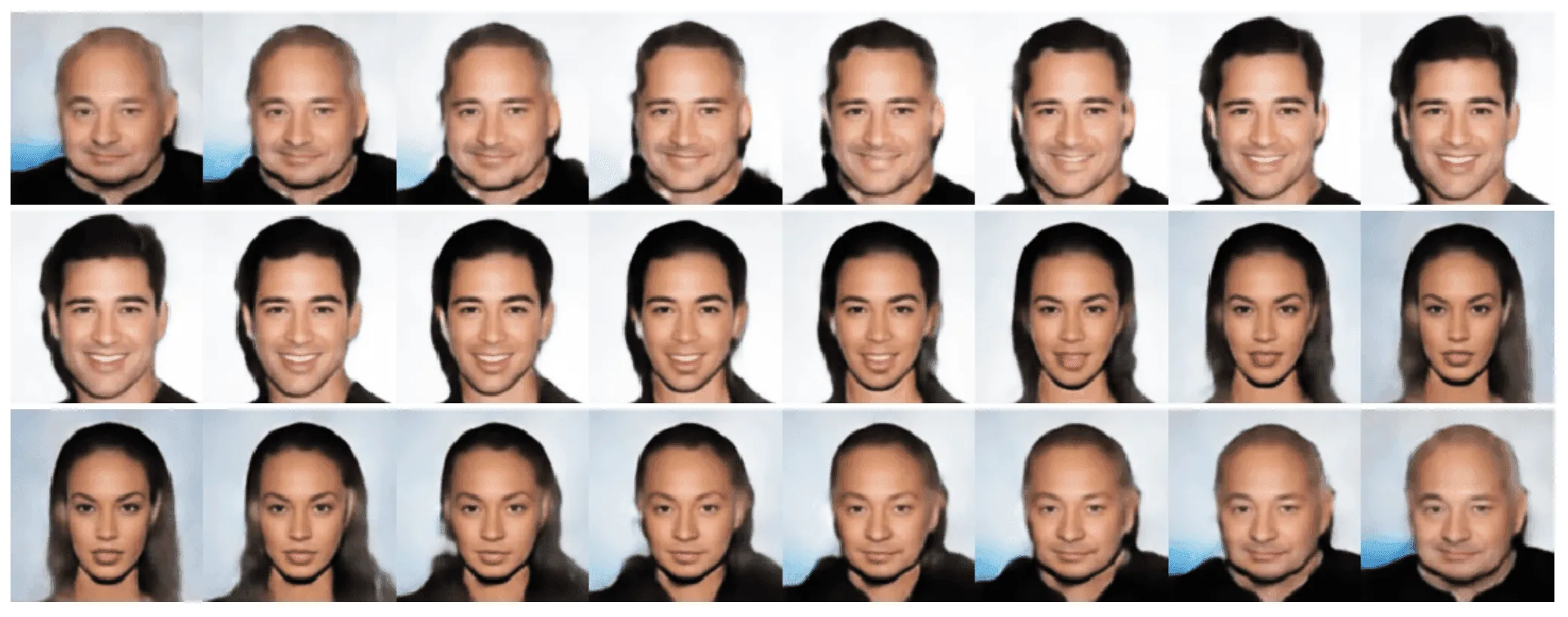
In the example above, we considered movement along a straight line, but in practice, interpolation can follow a more complex trajectory.

Manipulations in the latent space allow not only for smooth transitions between objects but also for editing generated objects. Typically, in such cases, it is necessary to identify directions in the latent space that correspond to specific attributes of the generated objects.

For example, one could find a direction responsible for hair color or smiling expressions in human face generation. We will explore these methods in more detail in the sections dedicated to specific models.

Applications of Generative Models

Why would one need to generate new data or estimate its density? The simplest example is data augmentation, which helps prevent overfitting and improves the generalization ability of a model.

Simple data augmentations such as random shifts, rotations, scaling, color, and contrast adjustments are widely used in almost all machine learning methods. However, generative models provide a more advanced form of data augmentation that can significantly expand a dataset or enrich it with completely new elements.

For instance, a generative model that applies style transfer—transferring the style of one image onto another—can be used to train more robust classification models. In a study by Sandfort et al., generative neural networks were used for data augmentation to improve the quality of segmentation in CT scans.

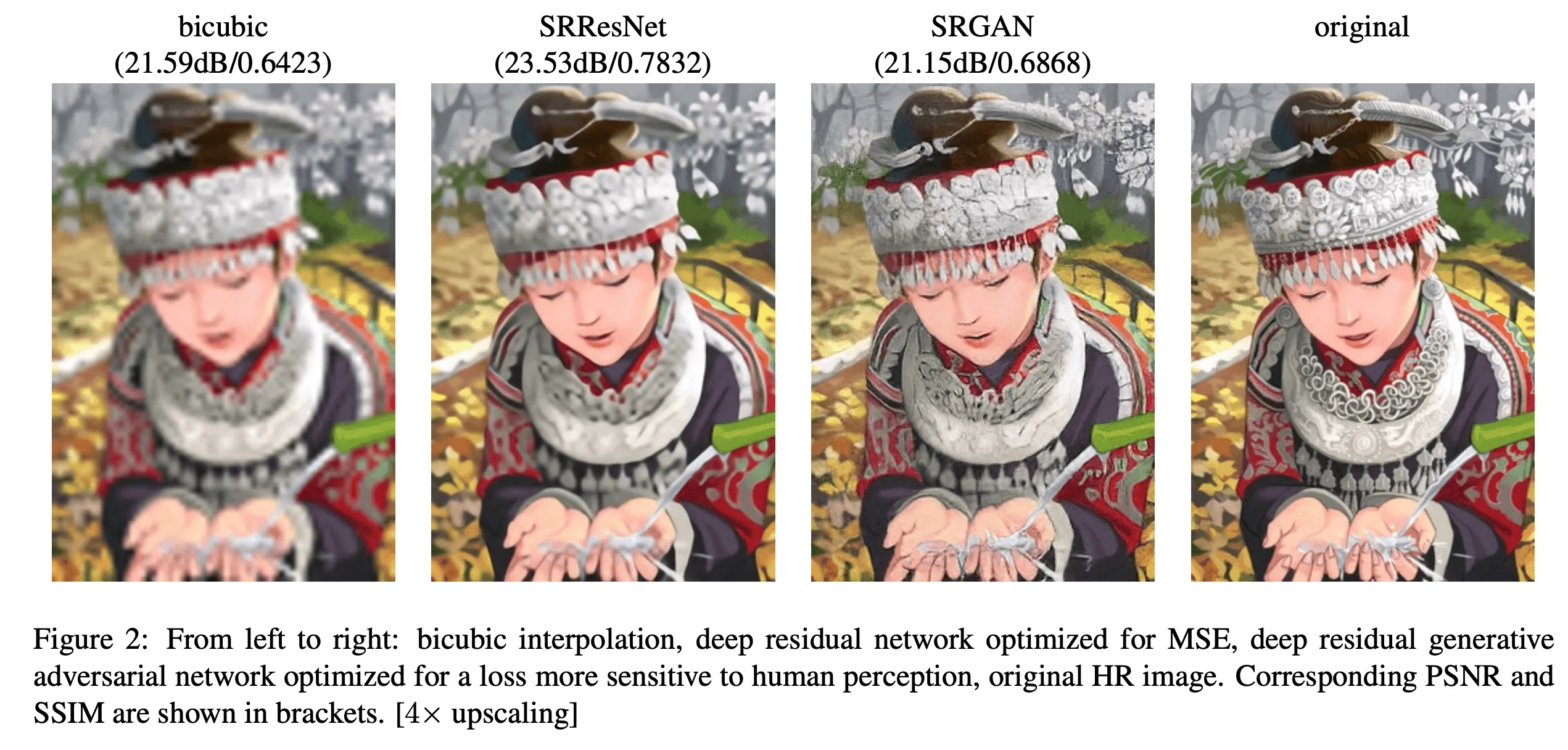
Additionally, generative models are widely applied in various image editing tasks. They are used to enhance image resolution, a problem known as super-resolution.

In the image below, the original picture (original) was first reduced in size by a factor of four and then restored to its original dimensions using different methods. It is evident that SRGAN—a method based on Generative Adversarial Networks (GANs)—performs significantly better than the traditional bicubic interpolation method, which often results in a blurry image.

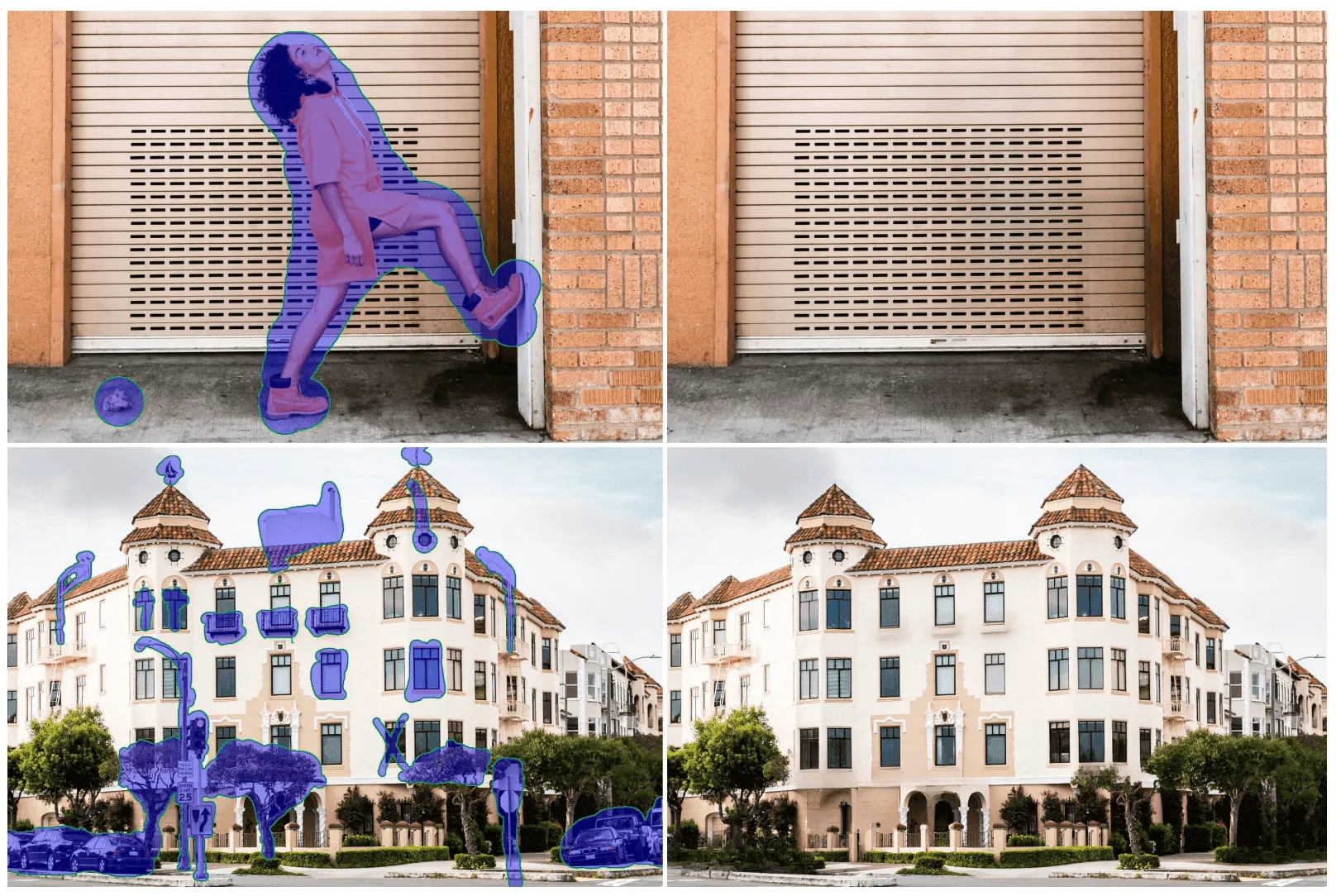
Generative models can be used to fill in missing parts of images. This is particularly useful when we want to remove unwanted objects or people from a photo and need to seamlessly fill the empty spaces left after their removal. This feature is already available in some modern smartphones.

In recent years, models that generate images based on textual descriptions have significantly improved. Some of the most well-known models include:

• Stable Diffusion – Open-source model. GitHub
• DALLE 2 – Available via a paid API. More Info
• Midjourney – Available via Discord. Official Site
• Imagen – A text-to-image model by Google AI. More Info

There are now dedicated databases for AI-generated images: Lexica and Openart.

The availability of such models has led to numerous applications, including:

• Illustrations for books – Example on Reddit
• Logo creation – Case study using DALL·E 2
• Interior design – AI-generated room designs
• Tattoo generation – AI-powered tattoo designs

Additionally, some models allow combining multiple tasks, such as inpainting based on text descriptions. For example, removing an object from an image and instructing the model on what should be drawn in its place.

Based on this technology, several image editors with built-in generative models have emerged:

• Neural Love – AI-enhanced image editing
• Photoroom – Background remover and AI editor
• ZMO – AI image generation and enhancement

Modern generative models have achieved remarkable quality and are now being actively used in real-world applications, as we have described throughout this section.

Generative adversarial networks

Introduction

Generative Adversarial Networks (GANs) are a broad class of generative models that are trained alongside another network that attempts to distinguish generated objects from real ones.

In this section, we will cover the fundamentals of GANs, provide an intuitive explanation of their working principles, and explore numerous techniques and modifications that enhance the original approach in the most successful models.

Additionally, we will showcase various practical applications where Generative Adversarial Networks have been effectively utilized.

The simplest and most effective design of generative models that can only sample but not estimate density is the transformation of one set of random variables into another.

Fundamentals of GAN Training

Generative Adversarial Networks (GANs) are implicit generative models. This means they do not explicitly estimate the probability density of the data but instead learn to sample from the data distribution.

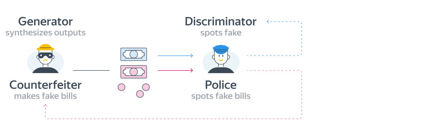
A classical analogy for how GANs learn is the scenario of a counterfeiter and a policeman. The counterfeiter's goal is to create counterfeit banknotes that the policeman cannot distinguish from real ones. The policeman's task is to learn how to differentiate the counterfeit banknotes from the authentic ones.

To understand how GANs train, imagine the following thought experiment: Suppose the counterfeiter and the policeman are friends who decide to improve their skills together. The counterfeiter creates several fake banknotes and shows them to the policeman. The policeman then evaluates them and informs the counterfeiter which ones he thinks are fake and which ones appear real. The counterfeiter remembers this feedback and improves the fake banknotes accordingly for the next round. At the same time, the policeman also learns: he keeps track of the fake notes he has seen to refine his ability to distinguish real from fake.

Imagine that this process repeats multiple times. What happens as a result? Each time, the counterfeiter produces banknotes that become harder and harder to differentiate from real ones. Similarly, the policeman's ability to detect counterfeit money improves continuously.

The key question for understanding GANs: At what point can we say that the counterfeiter is truly skilled at forging banknotes?

The answer: When the counterfeiter is able to fool even a highly trained policeman. At the beginning of the experiment, the policeman may not be very skilled at detecting counterfeits, so low-quality fake banknotes might deceive him. However, our ultimate goal is to develop a counterfeiter who can produce banknotes that are indistinguishable from the original ones, even for a professional expert.

While GANs are powerful, they come with several challenges:

• Mode Collapse: The generator may learn to produce limited variations of outputs instead of generating diverse samples.
• Training Instability: The generator and discriminator must remain balanced—if one improves too quickly, the other may fail to learn.
• Vanishing Gradients: If the discriminator becomes too good, the generator may stop receiving meaningful feedback for improvement.

To address these challenges, researchers have introduced various modifications to the standard GAN framework:

• Wasserstein GAN (WGAN): Improves stability by changing the loss function, making training more efficient.
• Conditional GAN (cGAN): Allows control over the generated output by conditioning on additional input (e.g., class labels).
• StyleGAN: Used for high-quality image generation, particularly in human face synthesis.
• CycleGAN: Enables image-to-image translation without paired training data (e.g., converting horse images to zebra images).

Applications of GANs

GANs have numerous real-world applications, including:

• Image Synthesis: Generating realistic human faces, artwork, and objects.
• Data Augmentation: Enhancing datasets for training machine learning models.
• Style Transfer: Applying artistic styles to photos or modifying image features.
• Super-Resolution: Enhancing low-resolution images to improve detail and clarity.
• Deepfake Technology: Replacing faces in videos with AI-generated counterparts.

GANs demonstrated that an adversarial objective can produce highly realistic synthetic data and remain important in areas such as image translation and controllable synthesis. Their unstable training and limited mode coverage also help explain why other generative approaches are often preferred for general-purpose generation today.